����ѧϰ��ѧ����
�ߵ���ѧ�����Դ���
-
�ݶ�����
- �ݶȵı�����һ������(ʸ��),��ʾijһ�����ڸõ㴦�ķ��������Ÿ÷���ȡ�����ֵ,�������ڸõ㴦���Ÿ÷���(���ݶȵķ���)�仯���,�仯�����(Ϊ���ݶȵ�ģ)
-
�ſ˱Ⱦ���(Jacobian����)
���� F : R n �� R m F: \mathbb{R}_{n} \rightarrow \mathbb{R}_{m} F:Rn?��Rm? ��һ����nάŷ�Ͽռ�ӳ�䵽��mάŷ�Ͽռ�ĺ�����
���������m��ʵ�������: y 1 ( x 1 , ? ? , x n ) , ? ? , y m ( x 1 , ? ? , x n ) y_{1}\left(x_{1}, \cdots, x_{n}\right), \cdots, y_{m}\left(x_{1}, \cdots, x_{n}\right) y1?(x1?,?,xn?),?,ym?(x1?,?,xn?) ��Щ������ƫ����(�������)�������һ��m��n�еľ���,������������ν���ſɱȾ���:
[ ? y 1 ? x 1 ? ? y 1 ? x n ? ? ? ? y m ? x 1 ? ? y m ? x n ] \left[\begin{array}{ccc} \frac{\partial y_{1}}{\partial x_{1}} & \cdots & \frac{\partial y_{1}}{\partial x_{n}} \\ \vdots & \ddots & \vdots \\ \frac{\partial y_{m}}{\partial x_{1}} & \cdots & \frac{\partial y_{m}}{\partial x_{n}} \end{array}\right] ?????x1??y1????x1??ym????????xn??y1????xn??ym???????
�ɼ�,�ݶ��������ſ˱Ⱦ��������! -
��ɭ����(Hessian Matrix),��һ����Ԫ�����Ķ���ƫ�������ɵķ���,�����˺����ľֲ����ʡ�����ѧ��,��ɭ������һ���Ա���Ϊ������ʵֵ�����Ķ���ƫ������ɵķ������
���O��һʵ������
f ( x 1 , x 2 , �� , x n ) f\left(x_{1}, x_{2}, \ldots, x_{n}\right) f(x1?,x2?,��,xn?)
��� f f f ���еĶ���ƫ����������,��ô f f f �ĺ�ɭ����ĵ� i j i j ij ��,��:
H ( f ) i j ( x ) = D i D j f ( x ) H(f)_{i j}(x)=D_{i} D_{j} f(x) H(f)ij?(x)=Di?Dj?f(x)
���� x = ( x 1 , x 2 , �� , x n ) , x=\left(x_{1}, x_{2}, \ldots, x_{n}\right), x=(x1?,x2?,��,xn?), ��
H ( f ) = [ ? 2 f ? x 1 2 ? 2 f ? x 1 ? x 2 ? ? 2 f ? x 1 ? x n ? 2 f ? x 2 ? x 1 ? 2 f ? x 2 2 ? ? 2 f ? x 2 ? x n ? ? ? ? ? 2 f ? x n ? x 1 ? 2 f ? x n ? x 2 ? ? 2 f ? x n 2 ] H(f)=\left[\begin{array}{cccc} \frac{\partial^{2} f}{\partial x_{1}^{2}} & \frac{\partial^{2} f}{\partial x_{1} \partial x_{2}} & \cdots & \frac{\partial^{2} f}{\partial x_{1} \partial x_{n}} \\ \frac{\partial^{2} f}{\partial x_{2} \partial x_{1}} & \frac{\partial^{2} f}{\partial x_{2}^{2}} & \cdots & \frac{\partial^{2} f}{\partial x_{2} \partial x_{n}} \\ \vdots & \vdots & \ddots & \vdots \\ \frac{\partial^{2} f}{\partial x_{n} \partial x_{1}} & \frac{\partial^{2} f}{\partial x_{n} \partial x_{2}} & \cdots & \frac{\partial^{2} f}{\partial x_{n}^{2}} \end{array}\right] H(f)=?????????x12??2f??x2??x1??2f???xn??x1??2f???x1??x2??2f??x22??2f???xn??x2??2f????????x1??xn??2f??x2??xn??2f???xn2??2f??????????
ʵ����,Hessian�������ݶ�����g(x)���Ա���x���ſ˱Ⱦ��� -
����������
��n��Ԫʵ���� f ( x 1 , x 2 , ? ? , x n ) f\left(x_{1}, x_{2}, \cdots, x_{n}\right) f(x1?,x2?,?,xn?) �ڵ� M 0 ( a 1 , a 2 , �� , a n ) M_{0}\left(a_{1}, a_{2}, \ldots, a_{n}\right) M0?(a1?,a2?,��,an?) ���������ж�������ƫ��,����:
? f ? x j �O ( a 1 , a 2 , �� , a n ) = 0 , j = 1 , 2 , �� , n \left.\frac{\partial f}{\partial x_{j}}\right|_{\left(a_{1}, a_{2}, \ldots, a_{n}\right)}=0, j=1,2, \ldots, n ?xj??f?�O�O�O�O?(a1?,a2?,��,an?)?=0,j=1,2,��,n
����
A = [ ? 2 f ? x 1 2 ? 2 f ? x 1 ? x 2 ? ? 2 f ? x 1 ? x n ? 2 f ? x 2 ? x 1 ? 2 f ? x 2 2 ? ? 2 f ? x 2 ? x n ? ? ? ? ? 2 f ? x n ? x 1 ? 2 f ? x n ? x 2 ? ? 2 f ? x n 2 ] A=\left[\begin{array}{cccc} \frac{\partial^{2} f}{\partial x_{1}^{2}} & \frac{\partial^{2} f}{\partial x_{1} \partial x_{2}} & \cdots & \frac{\partial^{2} f}{\partial x_{1} \partial x_{n}} \\ \frac{\partial^{2} f}{\partial x_{2} \partial x_{1}} & \frac{\partial^{2} f}{\partial x_{2}^{2}} & \cdots & \frac{\partial^{2} f}{\partial x_{2} \partial x_{n}} \\ \vdots & \vdots & \ddots & \vdots \\ \frac{\partial^{2} f}{\partial x_{n} \partial x_{1}} & \frac{\partial^{2} f}{\partial x_{n} \partial x_{2}} & \cdots & \frac{\partial^{2} f}{\partial x_{n}^{2}} \end{array}\right] A=?????????x12??2f??x2??x1??2f???xn??x1??2f???x1??x2??2f??x22??2f???xn??x2??2f????????x1??xn??2f??x2??xn??2f???xn2??2f??????????
�������½��:
(1) ��A��������ʱ, f ( x 1 , x 2 , ? ? , x n ) f\left(x_{1}, x_{2}, \cdots, x_{n}\right) f(x1?,x2?,?,xn?) �� M 0 ( a 1 , a 2 , �� , a n ) M_{0}\left(a_{1}, a_{2}, \ldots, a_{n}\right) M0?(a1?,a2?,��,an?) ������Сֵ;
(2) ��A��������ʱ, f ( x 1 , x 2 , ? ? , x n ) f\left(x_{1}, x_{2}, \cdots, x_{n}\right) f(x1?,x2?,?,xn?) �� M 0 ( a 1 , a 2 , �� , a n ) M_{0}\left(a_{1}, a_{2}, \ldots, a_{n}\right) M0?(a1?,a2?,��,an?) ��������ֵ;
(3) ��A��������ʱ, M 0 ( a 1 , a 2 , �� , a n ) M_{0}\left(a_{1}, a_{2}, \ldots, a_{n}\right) M0?(a1?,a2?,��,an?) ���Ǽ�ֵ����
(4) ��AΪ������������븺������ʱ, M 0 ( a 1 , a 2 , �� , a n ) M_{0}\left(a_{1}, a_{2}, \ldots, a_{n}\right) M0?(a1?,a2?,��,an?) �ǡ�����"��ֵ��,����Ҫ���������������ж��� -
�����ʽԼ�����Ż����⡪���������ճ��ӷ�
-
�����ݶȵ��Ż����������ݶ��½���
-
�����ݶȵ��Ż���������ţ�ٵ�����
������������ͳ��
-
��Ҷ˹��ʽ
����:�� A 1 , A 2 , ? ? , A n A_{1}, A_{2}, \cdots, A_{n} A1?,A2?,?,An? ��һ�걸�¼���,�����һ�¼� B , P ( B ) > 0 , B, P(B)>0, B,P(B)>0, ��
P ( A i �O B ) = P ( A i B ) P ( B ) = P ( A i ) P ( B �O A i ) �� i = 1 n P ( A i ) P ( B �O A i ) P\left(A_{i} \mid B\right)=\frac{P\left(A_{i} B\right)}{P(B)}=\frac{P\left(A_{i}\right) P\left(B \mid A_{i}\right)}{\sum_{i=1}^{n} P\left(A_{i}\right) P\left(B \mid A_{i}\right)} P(Ai?�OB)=P(B)P(Ai?B)?=��i=1n?P(Ai?)P(B�OAi?)P(Ai?)P(B�OAi?)?
P ( A i ) P\left(A_{i}\right) P(Ai?) ����������ǰ���Ѿ�֪���ĸ���,����ϰ�ߵس�Ϊ������ʡ������������˴�Ʒ(�� B B B �� ��),��ʱ�������� P ( A i �O B ) P\left(A_{i} \mid B\right) P(Ai?�OB) ��ӳ���������Ժ�� B B B �����ġ���Դ��(����Ʒ����Դ)�ĸ��ֿ����ԵĴ�С,ͨ����Ϊ������ʡ� -
���ʷֲ�
-
����ֲ�:
P { X = k } = C n k p k ( 1 ? p ) n ? k P\{X=k\}=C_{n}^{k} p^{k}(1-p)^{n-k} P{X=k}=Cnk?pk(1?p)n?k -
���ɷֲ�:
P { X = k } = �� k k ! e ? �� , k = 0 , 1 , 2 , ? P\{X=k\}=\frac{\lambda^{k}}{k !} e^{-\lambda}, k=0,1,2, \cdots P{X=k}=k!��k?e?��,k=0,1,2,? -
��̬�ֲ�:
�����ܶȺ���:
f ( x ) = 1 2 �� �� e ? ( x ? �� ) 2 2 �� 2 f(x)=\frac{1}{\sqrt{2 \pi} \sigma} e^{-\frac{(x-\mu)^{2}}{2 \sigma^{2}}} f(x)=2��?��1?e?2��2(x?��)2?
���һ��������� ���Ӿ�ֵΪ �� , \mu, ��, ����Ϊ �� \sigma �� ����̬�ֲ�,��ѧ�ϼ���
X �� N ( �� , �� 2 ) X \sim N\left(\mu, \sigma^{2}\right) X��N(��,��2)
-
��ҵ
-
-
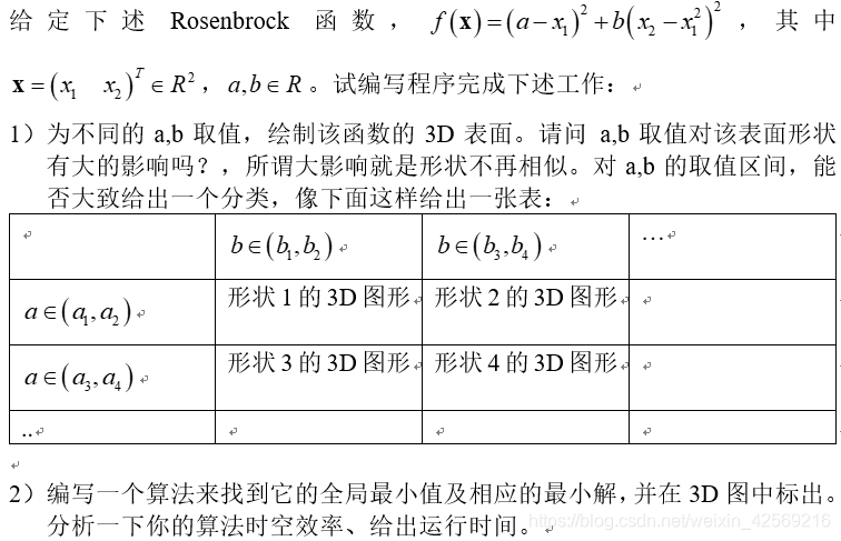
# encoding=gbk import numpy as np from mpl_toolkits.mplot3d import Axes3D import matplotlib.pyplot as plt from matplotlib import cm fig=plt.figure() ax = fig.add_subplot(projection='3d') x=np.arange(-1.5,1.5,0.005) # print(x) y=np.arange(-1.5,1.5,0.005) #���������������� x,y=np.meshgrid(x,y) # print(x) # print(y) def f(x,y): return (a - x) ** 2 + b * (y - x ** 2) ** 2 a = np.random.randint(1, 10) b = np.random.randint(10, 100) print((a, b)) #����3D���� ax.plot_surface(x,y,f(x,y),cmap = 'rainbow',) dic = {'a':a, 'b':b} ax.set_title(dic) ax.set_xlabel('X') ax.set_xlim(1.5, -1.5,) ax.set_ylabel('Y') ax.set_ylim(1.5, -1.5,) ax.set_zlabel('Z') plt.show()
-
![[����ͼƬת��ʧ��,Դվ�����з���������,���齫ͼƬ��������ֱ���ϴ�(img-2qW5uvtT-1626186074946)(C:\Users\xlli\AppData\Roaming\Typora\typora-user-images\image-20210713160222298.png)]](https://img-blog.csdnimg.cn/20210713222147399.png?x-oss-process=image/watermark,type_ZmFuZ3poZW5naGVpdGk,shadow_10,text_aHR0cHM6Ly9ibG9nLmNzZG4ubmV0L3dlaXhpbl80MjU2OTIxNg==,size_16,color_FFFFFF,t_70)
a��(1, 3),b��(1, 3)ʱ: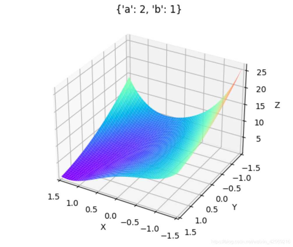
a��(1, 3),b��(6, 10)ʱ: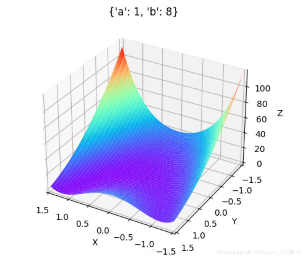
a��(6, 10),b��(1, 3)ʱ:
a��(6, 10),b��(6, 10)ʱ: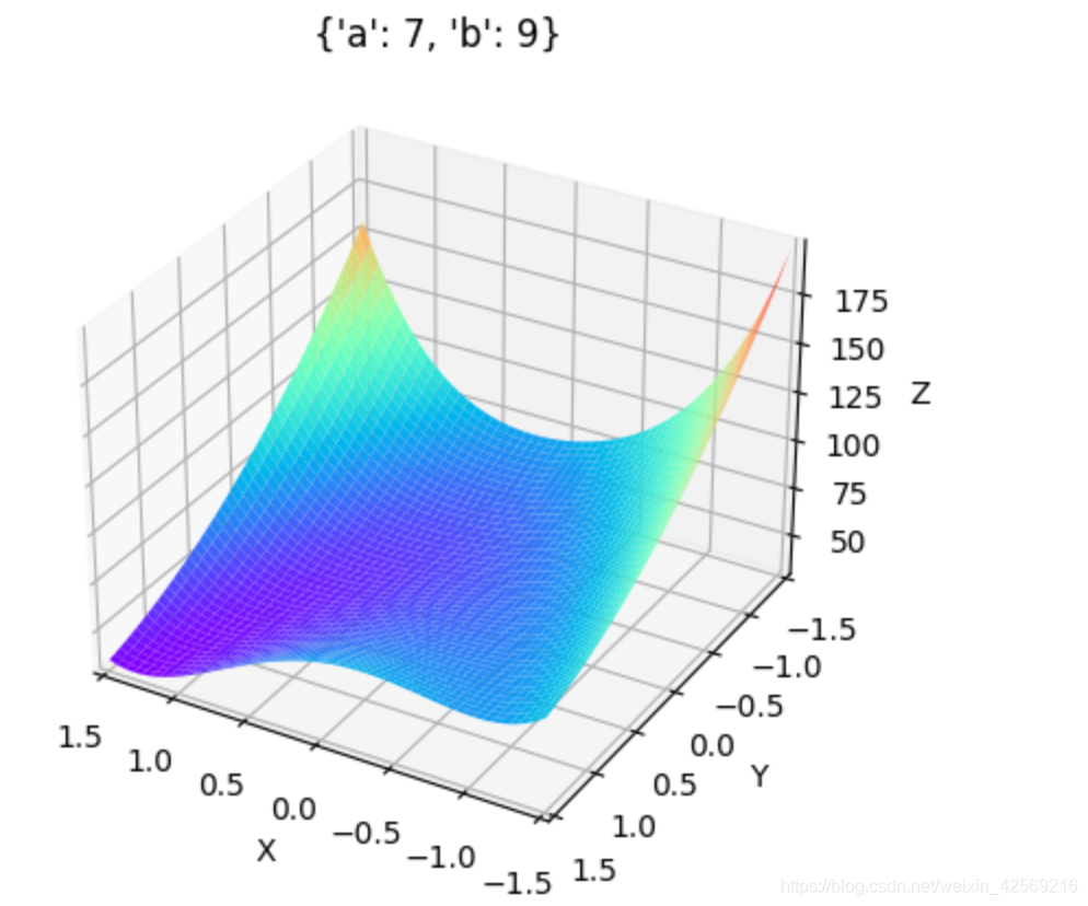
- ��ȫ����С��
�����
https://www.bilibili.com/video/BV1oQ4y1X7ep?p=2
https://github.com/datawhalechina/ensemble-learning