OpenCV学习的第三天,目的性是学习的最大动力,欲望则是目的的起源,坚持
第四节 图像金字塔(特征提取)
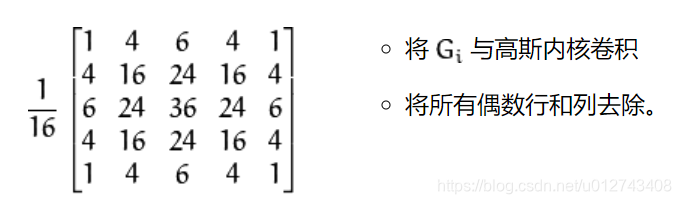
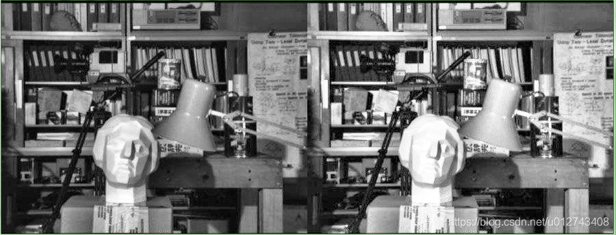
一、高斯金字塔:向下采样方法(缩小)
img=cv2.imread(“AM.png”)
cv_show(img,‘img’)
print (img.shape)
down=cv2.pyrDown(img)
cv_show(down,‘down’)
print (down.shape)
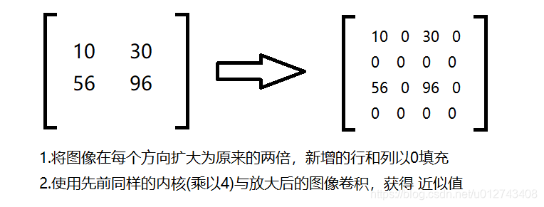
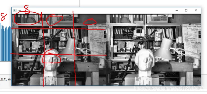
二、高斯金字塔:向上采样方法(放大)
img=cv2.imread(“AM.png”)
cv_show(img,‘img’)
print (img.shape)
up=cv2.pyrUp(img)
cv_show(up,‘up’)
print (up.shape)
第五节、拉普拉斯金字塔
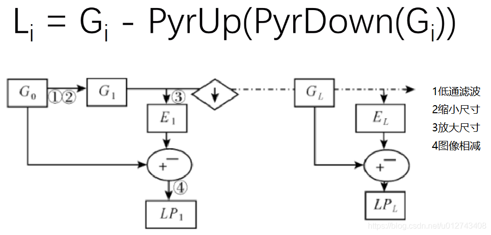
down=cv2.pyrDown(img)
down_up=cv2.pyrUp(down)
l_1=img-down_up
cv_show(l_1,‘l_1’)
第六节 图像轮廓(为了更高的准确率,使用二值图像。)
一、获取轮廓
cv2.findContours(img,mode,method)
mode:轮廓检索模式
- RETR_EXTERNAL :只检索最外面的轮廓;
- RETR_LIST:检索所有的轮廓,并将其保存到一条链表当中;
- RETR_CCOMP:检索所有的轮廓,并将他们组织为两层:顶层是各部分的外部边界,第二层是空洞的边界;
- RETR_TREE:检索所有的轮廓,并重构嵌套轮廓的整个层次;
method:轮廓逼近方法
- CHAIN_APPROX_NONE:以Freeman链码的方式输出轮廓,所有其他方法输出多边形(顶点的序列)。
- CHAIN_APPROX_SIMPLE:压缩水平的、垂直的和斜的部分,也就是,函数只保留他们的终点部分。

img = cv2.imread(‘contours.png’)
gray = cv2.cvtColor(img, cv2.COLOR_BGR2GRAY)
ret, thresh = cv2.threshold(gray, 127, 255, cv2.THRESH_BINARY)
cv_show(thresh,‘thresh’)
(二值图像)
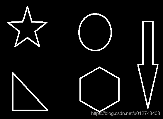
contours, hierarchy = cv2.findContours(thresh, cv2.RETR_TREE, cv2.CHAIN_APPROX_NONE)
np.array(contours).shape(保存的是轮廓信息)(11,)
hierarchy :层级
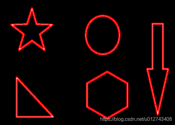
draw_img = img.copy() #注意需要copy,要不原图会变。。。
res = cv2.drawContours(draw_img, contours, -1, (0, 0, 255), 2) #传入绘制图像,轮廓,轮廓索引(-1表示所有),颜色模式(BGR),线条厚度
cv_show(res,‘res’)
二、轮廓特征
cnt = contours[0](获取轮廓)
cv2.contourArea(cnt)(计算轮廓面积)
cv2.arcLength(cnt,True)(计算轮廓周长)
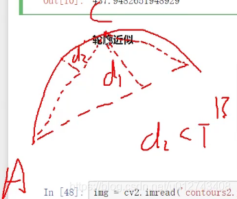
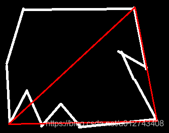
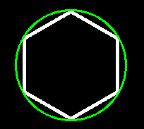
三、轮廓近似
img = cv2.imread(‘contours2.png’)
gray = cv2.cvtColor(img, cv2.COLOR_BGR2GRAY)
ret, thresh = cv2.threshold(gray, 127, 255, cv2.THRESH_BINARY)
binary, contours, hierarchy = cv2.findContours(thresh, cv2.RETR_TREE, cv2.CHAIN_APPROX_NONE)
cnt = contours[0]
draw_img = img.copy()
res = cv2.drawContours(draw_img, [cnt], -1, (0, 0, 255), 2)
cv_show(res,‘res’)
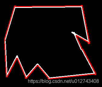
epsilon = 0.15*cv2.arcLength(cnt,True) (周长设定近似阈值)
approx = cv2.approxPolyDP(cnt,epsilon,True)
draw_img = img.copy()
res = cv2.drawContours(draw_img, [approx], -1, (0, 0, 255), 2)
cv_show(res,‘res’)
import cv2
import matplotlib.pyplot as plt
import numpy as np
def cv_show(img,name):
cv2.imshow(name,img)
cv2.waitKey()
cv2.destroyAllWindows()
img = cv2.imread(‘contours2.png’)
gray = cv2.cvtColor(img, cv2.COLOR_BGR2GRAY)
ret, thresh = cv2.threshold(gray, 127, 255, cv2.THRESH_BINARY)
contours, hierarchy = cv2.findContours(thresh, cv2.RETR_TREE, cv2.CHAIN_APPROX_NONE)
cnt = contours[0]
draw_img = img.copy()
res = cv2.drawContours(draw_img, [cnt], -1, (0, 0, 255), 2)
cv_show(res,‘res’)
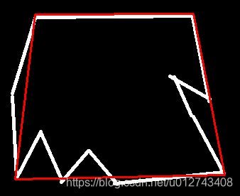
epsilon = 0.10*cv2.arcLength(cnt,True) (参数:越小,轮廓越近似本来形状)
approx = cv2.approxPolyDP(cnt,epsilon,True)
draw_img = img.copy()
res = cv2.drawContours(draw_img, [approx], -1, (0, 0, 255), 2)
cv_show(res,‘res’)
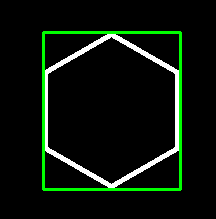
四、边界矩形、圆形
import cv2
import matplotlib.pyplot as plt
import numpy as np
def cv_show(img,name):
cv2.imshow(name,img)
cv2.waitKey()
cv2.destroyAllWindows()
img = cv2.imread(‘contours.png’)
gray = cv2.cvtColor(img, cv2.COLOR_BGR2GRAY)
ret, thresh = cv2.threshold(gray, 127, 255, cv2.THRESH_BINARY)
contours, hierarchy = cv2.findContours(thresh, cv2.RETR_TREE, cv2.CHAIN_APPROX_NONE)
cnt = contours[2]
x,y,w,h = cv2.boundingRect(cnt)
img = cv2.rectangle(img,(x,y),(x+w,y+h),(0,255,0),2)
cv_show(img,‘img’)
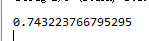
area = cv2.contourArea(cnt)
x, y, w, h = cv2.boundingRect(cnt)
rect_area = w * h
extent = float(area) / rect_area
print (‘轮廓面积与边界矩形比’,extent)
import cv2
import matplotlib.pyplot as plt
import numpy as np
def cv_show(img,name):
cv2.imshow(name,img)
cv2.waitKey()
cv2.destroyAllWindows()
img = cv2.imread(‘contours.png’)
gray = cv2.cvtColor(img, cv2.COLOR_BGR2GRAY)
ret, thresh = cv2.threshold(gray, 127, 255, cv2.THRESH_BINARY)
contours, hierarchy = cv2.findContours(thresh, cv2.RETR_TREE, cv2.CHAIN_APPROX_NONE)
cnt = contours[2]
(x,y),radius = cv2.minEnclosingCircle(cnt)
center = (int(x),int(y))
radius = int(radius)
img = cv2.circle(img,center,radius,(0,255,0),2)
cv_show(img,‘img’)
area = cv2.contourArea(cnt)
x, y, w, h = cv2.boundingRect(cnt)
rect_area = radius * radius*3.14
extent = float(area) / rect_area
print(extent)
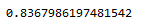
第七节、模板匹配
模板匹配和卷积原理很像,模板在原图像上从原点开始滑动,计算模板与(图像被模板覆盖的地方)的差别程度,这个差别程度的计算方法在opencv里有6种,然后将每次计算的结果放入一个矩阵里,作为结果输出。假如原图形是AxB大小,而模板是axb大小,则输出结果的矩阵是(A-a+1)x(B-b+1)
- TM_SQDIFF:计算平方不同,计算出来的值越小,越相关
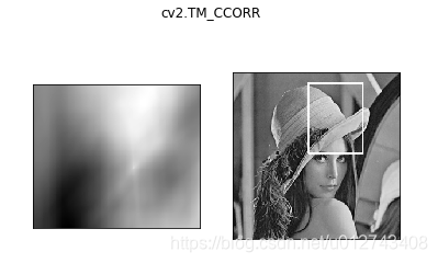
- TM_CCORR:计算相关性,计算出来的值越大,越相关
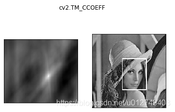
- TM_CCOEFF:计算相关系数,计算出来的值越大,越相关
- TM_SQDIFF_NORMED:计算归一化平方不同,计算出来的值越接近0,越相关
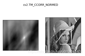
- TM_CCORR_NORMED:计算归一化相关性,计算出来的值越接近1,越相关
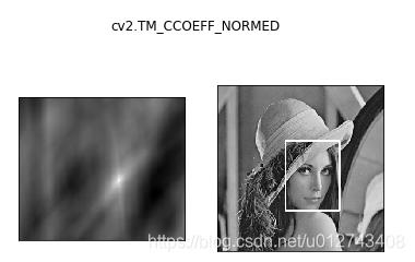
- TM_CCOEFF_NORMED:计算归一化相关系数,计算出来的值越接近1,越相关
(推荐使用归一化,计算精确度高,相对比较公平)
img = cv2.imread(‘lena.jpg’, 0)
template = cv2.imread(‘face.jpg’, 0)
img.shape((263, 263))
template.shape((110, 85))
res = cv2.matchTemplate(img, template, cv2.TM_SQDIFF)
res.shape((154, 179))
min_val, max_val, min_loc, max_loc = cv2.minMaxLoc(res)(最小值,最大值,最小值坐标位置,最大值坐标位置)
根据所用的算法,去找最值(精确度高),然后根据W,H找到匹配位置
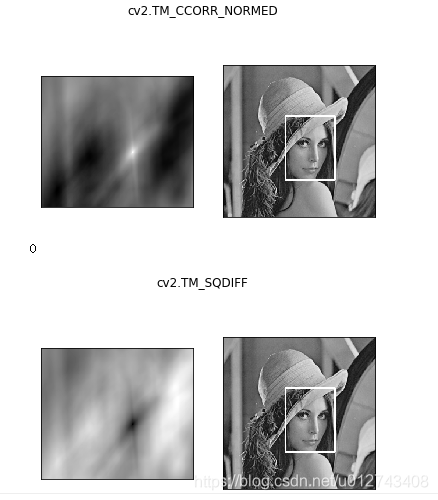
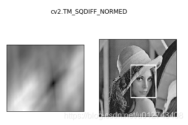
methods = [‘cv2.TM_CCOEFF’, ‘cv2.TM_CCOEFF_NORMED’, ‘cv2.TM_CCORR’,
‘cv2.TM_CCORR_NORMED’, ‘cv2.TM_SQDIFF’, ‘cv2.TM_SQDIFF_NORMED’]
for meth in methods:
img2 = img.copy()
# 匹配方法的真值
method = eval(meth)
print (method)
res = cv2.matchTemplate(img, template, method)
min_val, max_val, min_loc, max_loc = cv2.minMaxLoc(res)

# 如果是平方差匹配TM_SQDIFF或归一化平方差匹配TM_SQDIFF_NORMED,取最小值
if method in [cv2.TM_SQDIFF, cv2.TM_SQDIFF_NORMED]:
    top_left = min_loc
else:
    top_left = max_loc
bottom_right = (top_left[0] + w, top_left[1] + h)

# 画矩形
cv2.rectangle(img2, top_left, bottom_right, 255, 2)

plt.subplot(121), plt.imshow(res, cmap='gray')
plt.xticks([]), plt.yticks([])  # 隐藏坐标轴
plt.subplot(122), plt.imshow(img2, cmap='gray')
plt.xticks([]), plt.yticks([])
plt.suptitle(meth)
plt.show()
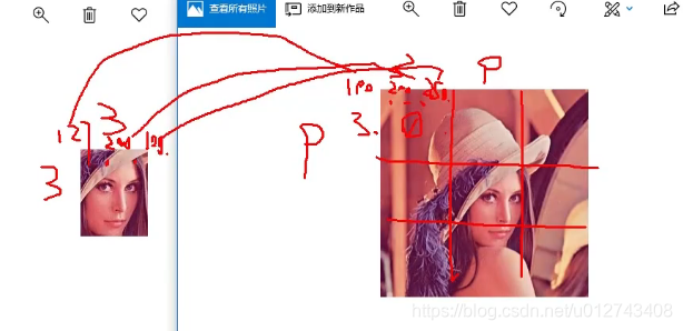
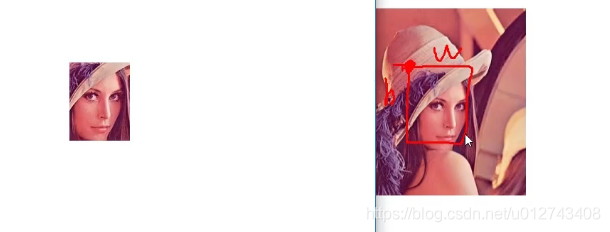
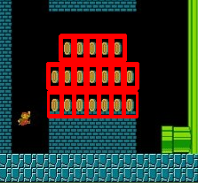
二、匹配多个对象
import cv2
import matplotlib.pyplot as plt
import numpy as np
def cv_show(img,name):
cv2.imshow(name,img)
cv2.waitKey()
cv2.destroyAllWindows()
img_rgb = cv2.imread(‘mario.jpg’)
img_gray=cv2.cvtColor(img_rgb,cv2.COLOR_BGR2GRAY)
template = cv2.imread(‘mario_coin.jpg’, 0)
h, w = template.shape[:2]
res = cv2.matchTemplate(img_gray, template, cv2.TM_CCOEFF_NORMED)
threshold = 0.8
loc = np.where(res >= threshold)
for pt in zip(*loc[::-1]):
bottom_right = (pt[0] + w, pt[1] + h)
cv2.rectangle(img_rgb, pt, bottom_right, (0, 0, 255), 2)
cv2.imshow(‘img_rgb’, img_rgb)
cv2.waitKey(0)
第八节、直方图
一、绘制图片像素点直方图
统计图片像素点
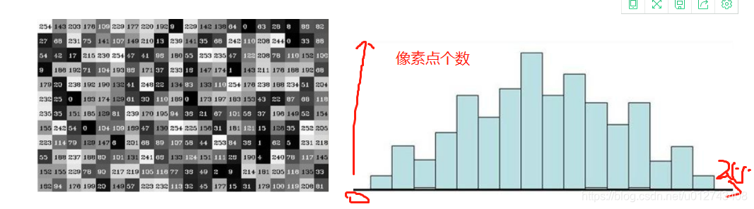
cv2.calcHist(images,channels,mask,histSize,ranges)
- images: 原图像图像格式为 uint8 或 ?oat32。当传入函数时应 用中括号 [] 括来例如[img]
- channels: 同样用中括号括来它会告函数我们统幅图 像的直方图。如果入图像是灰度图它的值就是 [0]
-
如果是彩色图像 的传入的参数可以是 [0][1][2] 它们分别对应着 BGR。 - mask: 掩模图像。统整幅图像的直方图就把它为 None。但是如 果你想统图像某一分的直方图的你就制作一个掩模图像并 使用它。
- histSize:BIN 的数目。也应用中括号括来
- ranges: 像素值范围常为 [0256]
import cv2
import matplotlib.pyplot as plt
import numpy as np
def cv_show(img,name):
cv2.imshow(name,img)
cv2.waitKey()
cv2.destroyAllWindows()
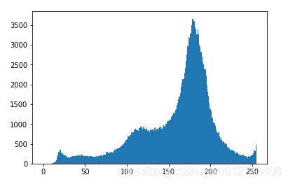
img = cv2.imread(‘cat.jpg’,0)
plt.hist(img.ravel(),256);
plt.show()
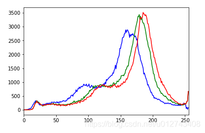
img = cv2.imread(‘cat.jpg’)
color = (‘b’,‘g’,‘r’)
for i,col in enumerate(color):
histr = cv2.calcHist([img],[i],None,[256],[0,256])
plt.plot(histr,color = col)
plt.xlim([0,256])
plt.show()
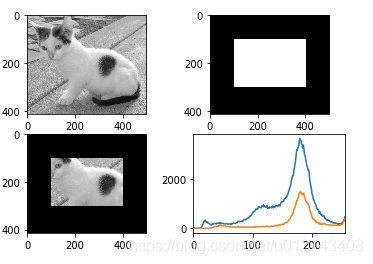
二、mask操作(与操作)
mask = np.zeros(img.shape[:2], np.uint8)
print (mask.shape)
mask[100:300, 100:400] = 255
cv_show(mask,‘mask’)
img = cv2.imread(‘cat.jpg’, 0)
cv_show(img,‘img’)
masked_img = cv2.bitwise_and(img, img, mask=mask)
cv_show(masked_img,‘masked_img’)
hist_full = cv2.calcHist([img], [0], None, [256], [0, 256])
hist_mask = cv2.calcHist([img], [0], mask, [256], [0, 256])
plt.subplot(221), plt.imshow(img, ‘gray’)
plt.subplot(222), plt.imshow(mask, ‘gray’)
plt.subplot(223), plt.imshow(masked_img, ‘gray’)
plt.subplot(224), plt.plot(hist_full), plt.plot(hist_mask)
plt.xlim([0, 256])
plt.show()
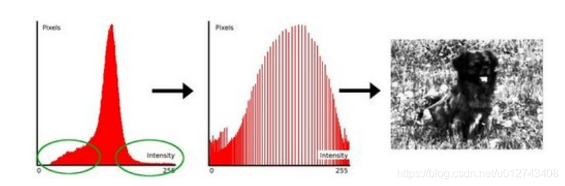
第九节、直方图均衡化(均衡化直方图可以提升图片的亮度、色彩)
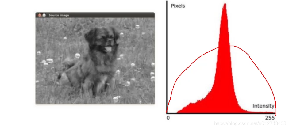
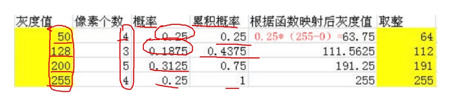
原图的像素直方图根据各个像素值及像素值个数,计算概率,根据概率计算累计概率,然后根据函数映射后获取新的像素值
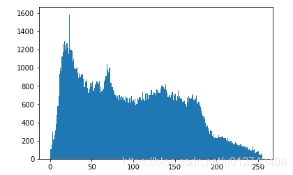
原图直方图
img = cv2.imread(‘clahe.jpg’,0) #0表示灰度图 #clahe
plt.hist(img.ravel(),256);
plt.show()
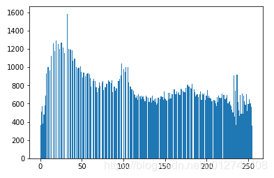
均衡后直方图
equ = cv2.equalizeHist(img)
plt.hist(equ.ravel(),256)
plt.show()
均衡后图片显示
res = np.hstack((img,equ))
cv_show(res,‘res’)
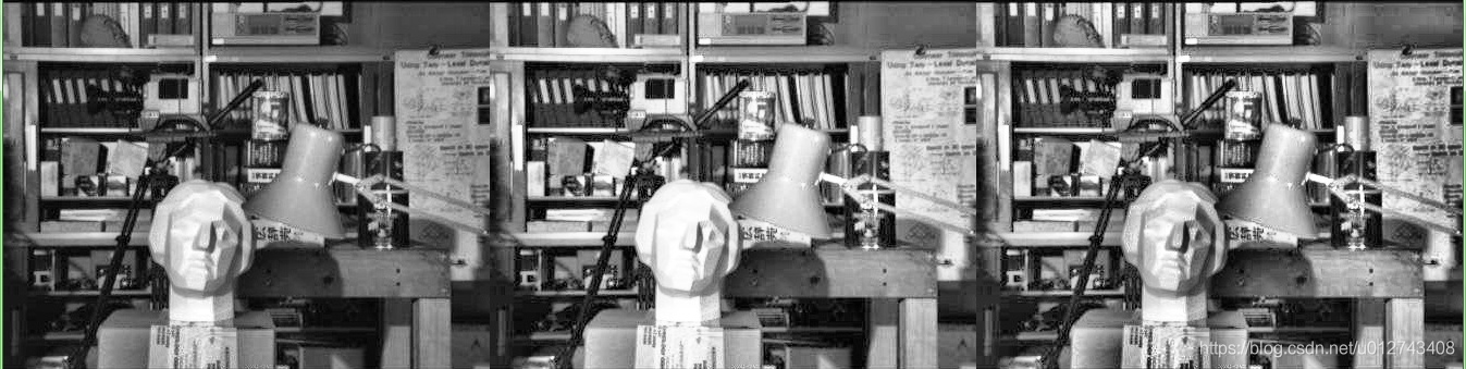
自适应均衡化
clahe = cv2.createCLAHE(clipLimit=2.0, tileGridSize=(8,8))
res_clahe = clahe.apply(img)
res = np.hstack((img,equ,res_clahe))
cv_show(res,‘res’)
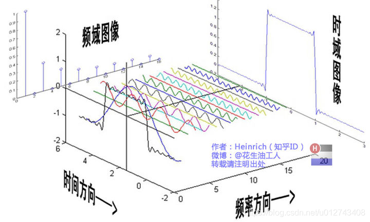
第十节、傅里叶变换(https://zhuanlan.zhihu.com/p/19763358)
以时间作为参照来观察动态世界的方法我们称其为时域分析,但是在频域中一切都是静止的,任何周期函数,都可以看作是不同振幅,不同相位正弦波的叠加
一、傅里叶变换的作用
高频:变化剧烈的灰度分量,例如边界
低频:变化缓慢的灰度分量,例如一片大海
滤波
低通滤波器:只保留低频,会使得图像模糊
高通滤波器:只保留高频,会使得图像细节增强
1、输入图像需要先转换成np.float32 格式
img = cv2.imread(‘lena.jpg’,0)
img_float32 = np.float32(img)
2、得到的结果中频率为0的部分会在左上角,通常要转换到中心位置,可以通过shift变换来实现
dft = cv2.dft(img_float32, flags = cv2.DFT_COMPLEX_OUTPUT)
dft_shift = np.fft.fftshift(dft)
3、cv2.dft()返回的结果是双通道的(实部,虚部),通常还需要转换成图像格式才能展示(0,255)
得到灰度图能表示的形式
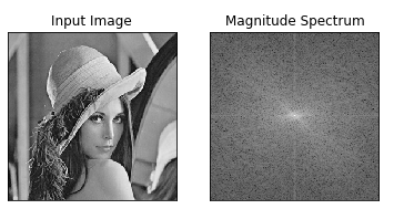
magnitude_spectrum = 20*np.log(cv2.magnitude(dft_shift[:,:,0],dft_shift[:,:,1]))
plt.subplot(121),plt.imshow(img, cmap = ‘gray’)
plt.title(‘Input Image’), plt.xticks([]), plt.yticks([])
plt.subplot(122),plt.imshow(magnitude_spectrum, cmap = ‘gray’)
plt.title(‘Magnitude Spectrum’), plt.xticks([]), plt.yticks([])
plt.show()
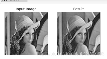
低通滤波器:
import numpy as np
import cv2
from matplotlib import pyplot as plt
img = cv2.imread(‘lena.jpg’,0)
img_float32 = np.float32(img)
dft = cv2.dft(img_float32, flags = cv2.DFT_COMPLEX_OUTPUT)
dft_shift = np.fft.fftshift(dft)
rows, cols = img.shape
crow, ccol = int(rows/2) , int(cols/2) # 中心位置
低通滤波
mask = np.zeros((rows, cols, 2), np.uint8)
mask[crow-30:crow+30, ccol-30:ccol+30] = 1
IDFT
fshift = dft_shift*mask
f_ishift = np.fft.ifftshift(fshift)
img_back = cv2.idft(f_ishift)
img_back = cv2.magnitude(img_back[:,:,0],img_back[:,:,1])
plt.subplot(121),plt.imshow(img, cmap = ‘gray’)
plt.title(‘Input Image’), plt.xticks([]), plt.yticks([])
plt.subplot(122),plt.imshow(img_back, cmap = ‘gray’)
plt.title(‘Result’), plt.xticks([]), plt.yticks([])
plt.show()
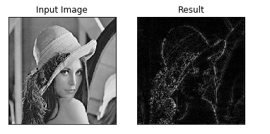
高通滤波器:
img = cv2.imread(‘lena.jpg’,0)
img_float32 = np.float32(img)
dft = cv2.dft(img_float32, flags = cv2.DFT_COMPLEX_OUTPUT)
dft_shift = np.fft.fftshift(dft)
rows, cols = img.shape
crow, ccol = int(rows/2) , int(cols/2) # 中心位置
高通滤波
mask = np.ones((rows, cols, 2), np.uint8)
mask[crow-30:crow+30, ccol-30:ccol+30] = 0
IDFT
fshift = dft_shift*mask
f_ishift = np.fft.ifftshift(fshift)
img_back = cv2.idft(f_ishift)
img_back = cv2.magnitude(img_back[:,:,0],img_back[:,:,1])
plt.subplot(121),plt.imshow(img, cmap = ‘gray’)
plt.title(‘Input Image’), plt.xticks([]), plt.yticks([])
plt.subplot(122),plt.imshow(img_back, cmap = ‘gray’)
plt.title(‘Result’), plt.xticks([]), plt.yticks([])
plt.show()