[人工智能]【Python】DS的基础学习笔记13：Scikit-learn库

Scikit-learn库

scikit-learn库是当今最流行的机器学习算法库之一
可用来解决分类与回归问题
以鸢尾花数据集为例，简单了解八大传统机器学习分类算法的sk-learn实现
欲深入了解传统机器学习算法的原理和公式推导，请继续学习《统计学习方法》或《西瓜书》

13.0 鸢尾花数据集

13.0.1 下载数据集

import seaborn as sns

iris = sns.load_dataset("iris")

13.0.2 数据集的查看

type(iris)

<class ‘pandas.core.frame.DataFrame’>

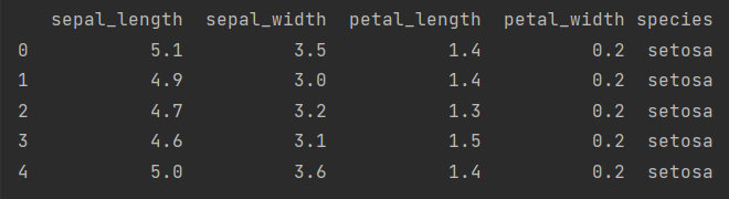
iris.head()

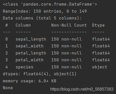
iris.info()

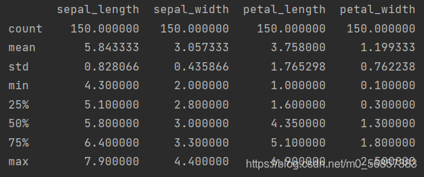
iris.describe()

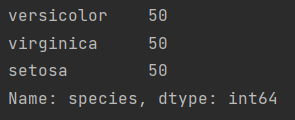
iris.species.value_counts()

sns.pairplot(data=iris, hue="species")
plt.show()

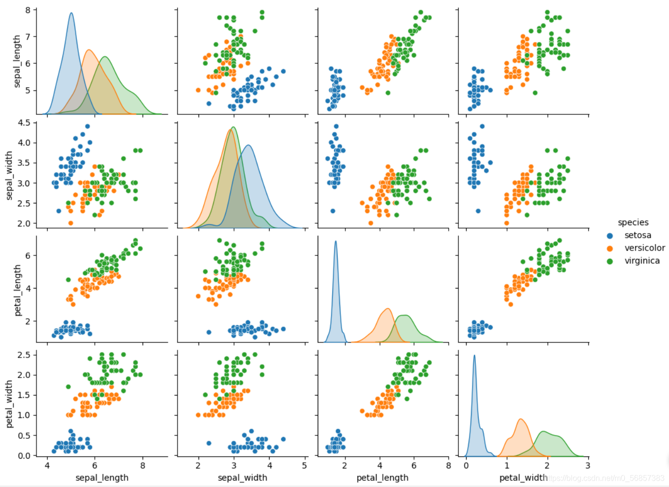
我们为了简化问题，决定研究花瓣petal长度与宽度来对鸢尾花进行分类
从而花萼sepal相关数据暂时不考虑

13.0.3 标签清洗

iris_simple = iris.drop(["sepal_length", "sepal_width"], axis=1)
iris_simple.head()

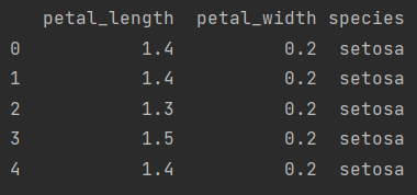
我们可以发现在species这一标签下的标签值为字符串类型，在分类算法中可能会利用到该标签值，我们需要将字符串类型编码为数字类型，方便后续处理，利用映射关系对其进行编码

13.0.4 标签编码

from sklearn.preprocessing import LabelEncoder

iris_simple["species"] = encoder.fit_transform(iris_simple["species"])
iris_simple

有时，我们会发现不同特征下的数据绝对值差异比较大，比如某列上千上万，而另一列都是0.1、0.2这种量级的，而在有的算法中数据绝对值比较大的特征会对整个结果影响更大一些，并且这种情况下会影响算法收敛速度
这种情况需要对数据进行标准化处理

13.0.5 数据集的标准化

PS：本数据集特征比较接近，不存在绝对值量级差异较大的情况，实际处理过程中未进行标准化

from sklearn.preprocessing import StandardScaler
import pandas as pd

trans = StandardScaler()
_iris_simple = trans.fit_transform(iris_simple[["petal_length", "petal_width"]])
_iris_simple = pd.DataFrame(_iris_simple, columns=["petal_length", "petal_width"])
_iris_simple.describe()

该原理为Z-score normalization
$$x_{normalization}=\frac{x?\mu }{\sigma }$$
也叫标准差标准化，经过处理的数据符合标准正态分布，即均值为 0，标准差为 1 。其中μ为所有样本数据的均值，σ为所有样本数据的标准差。
注意：计算时对每个特征分别进行。将数据按特征（按列进行）减去其均值，并除以其方差。得到的结果是，对于每个特征来说所有数据都聚集在0附近，方差为1。

但鸢尾花数据集中的特征绝对值相差不大，因此我们不对其进行标准化处理

13.0.6 构建训练集和测试集（暂不考虑验证集）

一般我们会把数据集分为三部分：训练集、验证集和测试集
训练集用来训练算法，得到收敛模型
验证集用来验证训练出来的算法是否足够优秀，通过不断调整我们的模型，来获得一个在验证集上表现比较好的一个模型
测试集是在我们经过很多次训练与验证之后得到我们认为较好的模型，判断其泛化能力是否足够的好

from sklearn.model_selection import train_test_split

train_set, test_set = train_test_split(iris_simple, test_size=0.2)  # test_size指测试集比例
test_set.head()

iris_x_train = train_set[["petal_length", "petal_width"]]  # 新的DataFrame对象与原来无关，无需copy
iris_x_train.head()

iris_y_train = train_set["species"].copy()  # 返回视图，需要copy
iris_y_train.head()

97 1
3 0
125 2
63 1
105 2
Name: species, dtype: int32

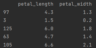
iris_x_test = test_set[["petal_length", "petal_width"]]
iris_x_test.head()

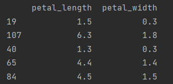
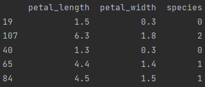
iris_y_test = test_set["species"].copy()
iris_y_test.head()

19 0
107 2
40 0
65 1
84 1
Name: species, dtype: int32

13.1 k近邻算法

13.1.1 基本思想

与待预测点最近的训练数据集中的k个邻居
把k个近邻中最常见的类别预测为待预测点的类别

13.1.2 sklearn实现

from sklearn.neighbors import KNeighborsClassifier

• 构建分类器对象

clf = KNeighborsClassifier()
clf

KNeighborsClassifier(algorithm=‘auto’, leaf_size=30, metric=‘minkowski’,
metric_params=None, n_jobs=None, n_neighbors=5, p=2,
weights=‘uniform’)

我们可以看到n_neighbors=5,因此该分类器默认k=5

• 训练

clf.fit(iris_x_train, iris_y_train)  # 训练

• 预测

res = clf.predict(iris_x_test)  # 预测
print(res)
print(iris_y_test.values)

[1 0 0 1 1 0 1 2 2 1 0 1 0 0 0 0 0 2 1 2 2 0 2 2 2 1 1 0 1 2]
[1 0 0 1 1 0 1 2 2 1 0 1 0 0 0 0 0 2 1 2 2 0 2 2 1 1 1 0 1 2]

• 翻转

encoder.inverse_transform(res)  # 翻转

[‘versicolor’ ‘setosa’ ‘setosa’ ‘versicolor’ ‘versicolor’ ‘setosa’
‘versicolor’ ‘virginica’ ‘virginica’ ‘versicolor’ ‘setosa’ ‘versicolor’
‘setosa’ ‘setosa’ ‘setosa’ ‘setosa’ ‘setosa’ ‘virginica’ ‘versicolor’
‘virginica’ ‘virginica’ ‘setosa’ ‘virginica’ ‘virginica’ ‘virginica’
‘versicolor’ ‘versicolor’ ‘setosa’ ‘versicolor’ ‘virginica’]

• 评估

accuracy = clf.score(iris_x_test, iris_y_test)  # 评估
print("预测正确率：{:.0%}".format(accuracy))

预测正确率：97%

• 存储数据

out = iris_x_test.copy()  # 存储数据
out["y"] = iris_y_test
out["pre"] = res
print(out)
out.to_csv("iris_predict.csv")

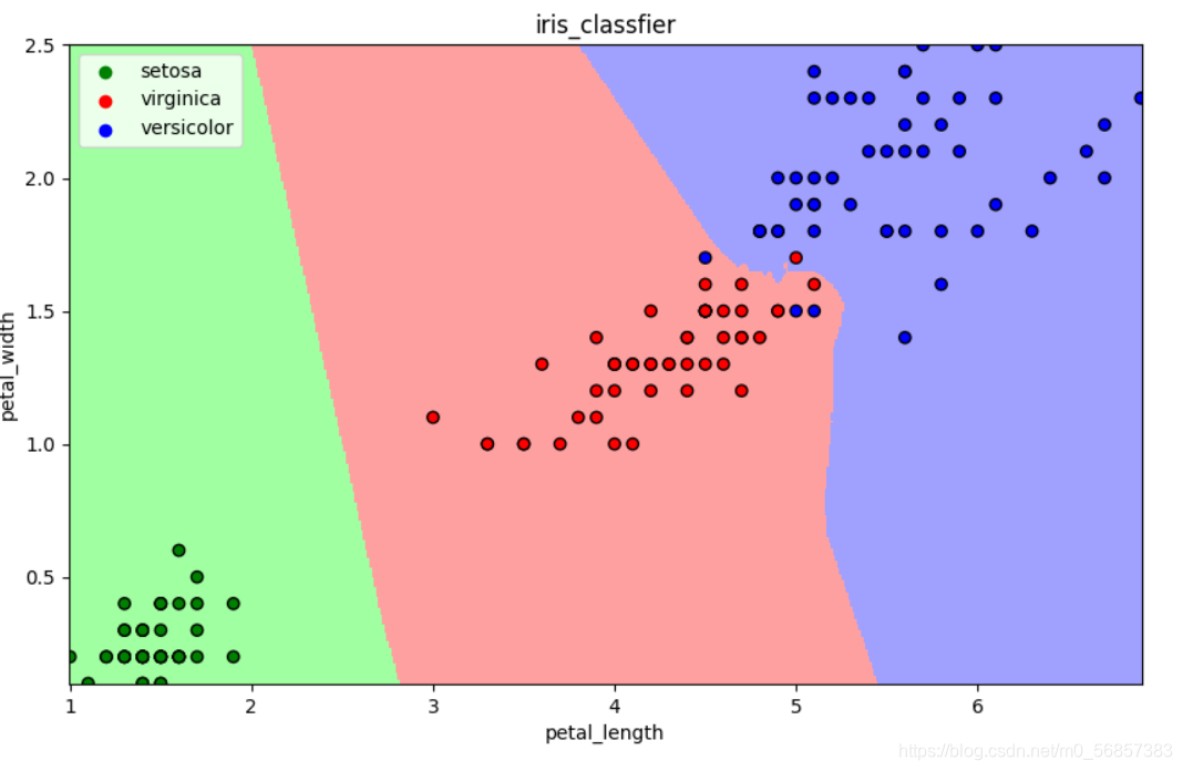
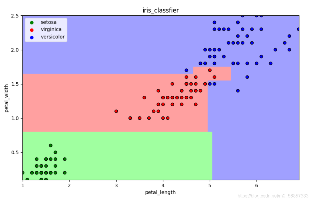
13.1.3 可视化

import numpy as np
import matplotlib as mpl
import matplotlib.pyplot as plt

def draw(clf):
    # 网格化
    M, N = 500, 500
    x1_min, x2_min = iris[["petal_length", "petal_width"]].min(axis=0)
    x1_max, x2_max = iris[["petal_length", "petal_width"]].max(axis=0)
    t1 = np.linspace(x1_min, x1_max, M)
    t2 = np.linspace(x2_min, x2_max, N)
    x1, x2 = np.meshgrid(t1, t2)

    # 预测
    x_show = np.stack((x1.flatten(), x2.flatten()), axis=1)
    y_predict = clf.predict(x_show)

    # 配色
    cm_light = mpl.colors.ListedColormap(["#A0FFA0", "#FFA0A0", "#A0A0FF"])
    cm_dark = mpl.colors.ListedColormap(["g", "r", "b"])

    # 绘制预测区域图
    plt.figure(figsize=(10, 6))
    plt.pcolormesh(x1, x2, y_predict.reshape(x1.shape), shading='auto', cmap=cm_light)

    # 绘制原始数据点
    plt.scatter(iris_simple["petal_length"], iris_simple["petal_width"], label=None,
                c=iris_simple["species"], cmap=cm_dark, marker='o', edgecolors="k")
    plt.xlabel("petal_length")
    plt.ylabel("petal_width")

    # 绘制图例
    color = ["g", "r", "b"]
    species = ["setosa", "virginica", "versicolor"]
    for i in range(3):
        plt.scatter([], [], c=color[i], label=species[i])  # 利用空点绘制图例
    plt.legend(loc="best")
    plt.title("iris_classfier")


draw(clf)
plt.show()

13.2 朴素贝叶斯算法

13.2.1 基本思想

当X=(x1, x2)发生的时候，哪一个yk发生的概率最大

13.2.2 sklearn实现

from sklearn.naive_bayes import GaussianNB

• 构建分类器对象

clf = GaussianNB()

• 训练

clf.fit(iris_x_train, iris_y_train)

• 预测

res = clf.predict(iris_x_test)
print(res)
print(iris_y_test.values)

[2 0 2 1 1 1 1 0 1 1 1 0 0 1 1 1 1 2 0 2 0 1 1 2 2 1 1 0 2 2]
[2 0 2 1 1 1 1 0 1 1 1 0 0 1 1 1 1 2 0 2 0 1 1 2 2 1 1 0 2 2]

• 评估

accuracy = clf.score(iris_x_test, iris_y_test)
print("预测正确率：{:.0%}".format(accuracy))

预测正确率：100%

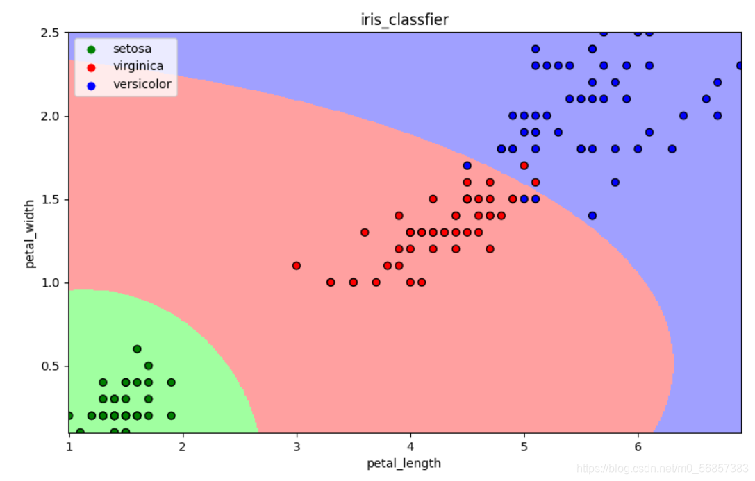
• 可视化

draw(clf)
plt.show()

13.3 决策树算法

13.3.1 基本思想

CART算法：每次通过一个特征，将数据尽可能地分为纯净的两类，递归地分下去

13.3.2 sklearn实现

from sklearn.tree import DecisionTreeClassifier

• 构建分类器对象

clf = DecisionTreeClassifier()
clf

DecisionTreeClassifier(class_weight=None, criterion=‘gini’, max_depth=None,
max_features=None, max_leaf_nodes=None,
min_impurity_decrease=0.0, min_impurity_split=None,
min_samples_leaf=1, min_samples_split=2,
min_weight_fraction_leaf=0.0, presort=False,
random_state=None, splitter=‘best’)

• 训练

clf.fit(iris_x_train, iris_y_train)

• 预测

res = clf.predict(iris_x_test)
print(res)
print(iris_y_test.values)

[1 1 1 1 1 0 1 2 1 0 0 2 2 0 0 1 2 0 0 1 0 1 1 2 2 2 0 2 1 1]
[1 1 1 1 1 0 1 2 1 0 0 2 2 0 0 1 2 0 0 1 0 1 1 2 2 2 0 2 1 1]

• 评估

accuracy = clf.score(iris_x_test, iris_y_test)
print("预测正确率:{:.0%}".format(accuracy))

预测正确率:100%

• 可视化

draw(clf)
plt.show()

13.4 逻辑回归算法

13.4.1 基本思想

一种解释：
训练：通过一个映射方式，将特征X=(x1, x2) 映射成P(y=ck)，求使得所有概率之积最大化地映射方式的参数
预测：计算P(y=ck)取概率最大的类别作为预测对象的分类

13.4.2 sklearn实现

from sklearn.linear_model import LogisticRegression

• 构建分类器对象

clf = LogisticRegression(solver="saga", max_iter=1000)  # 需要修改参数，默认参数分类效果不好

• 训练

clf.fit(iris_x_train, iris_y_train)
clf

LogisticRegression(C=1.0, class_weight=None, dual=False, fit_intercept=True,
intercept_scaling=1, l1_ratio=None, max_iter=1000,
multi_class=‘warn’, n_jobs=None, penalty=‘l2’,
random_state=None, solver=‘saga’, tol=0.0001, verbose=0,
warm_start=False)

• 预测

res = clf.predict(iris_x_test)
print(res)
print(iris_y_test.values)

[2 2 1 1 1 2 0 1 1 0 0 1 1 2 2 0 0 2 2 1 1 1 2 0 0 1 0 2 2 1]
[2 1 1 1 1 1 0 1 1 0 0 1 1 2 2 0 0 2 2 1 1 1 2 0 0 1 0 2 2 1]

• 评估

accuracy = clf.score(iris_x_test, iris_y_test)
print("预测正确率:{:.0%}".format(accuracy))

预测正确率:93%

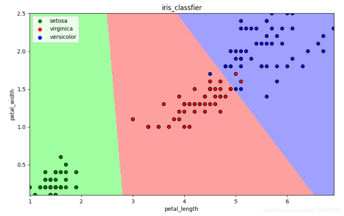
• 可视化

draw(clf)
plt.show()

13.5 支持向量机算法

13.5.1 基本思想

以二分类为例， 假设数据可以完全分开
用一个超平面将两类数据完全分开，且最近点到平面距离最大

13.5.2 sklearn实现

from sklearn.svm import SVC

• 构建分类器对象

clf = SVC()
clf

SVC(C=1.0, cache_size=200, class_weight=None, coef0=0.0,
decision_function_shape=‘ovr’, degree=3, gamma=‘auto_deprecated’,
kernel=‘rbf’, max_iter=-1, probability=False, random_state=None,
shrinking=True, tol=0.001, verbose=False)

• 训练

clf.fit(iris_x_train, iris_y_train)

• 预测

res = clf.predict(iris_x_test)
print(res)
print(iris_y_test.values)

[1 0 1 2 0 2 0 2 2 1 1 1 0 0 0 2 1 0 1 0 1 0 2 1 2 1 0 0 0 0]
[1 0 1 2 0 2 0 2 2 1 1 2 0 0 0 2 1 0 1 0 1 0 2 1 2 1 0 0 0 0]

• 评估

accuracy = clf.score(iris_x_test, iris_y_test)
print("预测正确率:{:.0%}".format(accuracy))

预测正确率:97%

• 可视化

draw(clf)
plt.show()

13.6 集成方法——随机森林

13.6.1 基本思想

训练集m，有放回的随机抽取m个数据，构成一组，共抽取n组采样集
n组采样集训练得到n个弱分类器，弱分类器一般用决策树或神经网络
将n个弱分类器进行组合得到强分类器

13.6.2 sklearn实现

from sklearn.ensemble import RandomForestClassifier

• 构建分类器对象

clf = RandomForestClassifier()
clf

RandomForestClassifier(bootstrap=True, class_weight=None, criterion=‘gini’,
max_depth=None, max_features=‘auto’, max_leaf_nodes=None,
min_impurity_decrease=0.0, min_impurity_split=None,
min_samples_leaf=1, min_samples_split=2,
min_weight_fraction_leaf=0.0, n_estimators=‘warn’,
n_jobs=None, oob_score=False, random_state=None,
verbose=0, warm_start=False)

• 训练

clf.fit(iris_x_train, iris_y_train)

• 预测

res = clf.predict(iris_x_test)
print(res)
print(iris_y_test.values)

[0 0 0 0 0 2 0 1 1 1 2 1 1 0 0 2 2 2 0 0 0 1 0 0 1 0 2 2 0 0]
[0 0 0 0 0 2 0 1 1 1 2 1 1 0 0 2 2 2 0 0 0 1 0 0 1 0 2 2 0 0]

• 评估

accuracy = clf.score(iris_x_test, iris_y_test)
print("预测正确率:{:.0%}".format(accuracy))

预测正确率:100%

• 可视化

draw(clf)
plt.show()

13.7 集成方法——Adaboost

13.7.1 基本思想

训练集m，用初始数据权重训练得到第一个弱分类器，根据误差率计算弱分类器系数，更新数据的权重
使用新的权重训练得到第二个弱分类器，以此类推
根据各自系数，将所有弱分类器加权求和获得强分类器

13.7.2 sklearn实现

from sklearn.ensemble import AdaBoostClassifier

• 构建分离器对象

clf = AdaBoostClassifier()
clf

AdaBoostClassifier(algorithm=‘SAMME.R’, base_estimator=None, learning_rate=1.0,
n_estimators=50, random_state=None)

• 训练

clf.fit(iris_x_train, iris_y_train)

• 预测

res = clf.predict(iris_x_test)
print(res)
print(iris_y_test.values)

[1 0 0 2 0 2 0 2 1 1 1 0 2 1 2 2 1 1 1 0 1 1 0 2 2 1 0 1 2 2]
[1 0 0 2 0 2 0 2 1 1 1 0 2 1 2 2 2 1 1 0 1 1 0 2 2 1 0 1 2 2]

• 评估

accuracy = clf.score(iris_x_test, iris_y_test)
print("预测正确率:{:.0%}".format(accuracy))

预测正确率:97%

• 可视化

draw(clf)
plt.show()

13.8 集成方法——梯度提升树GBDT

13.8.1 基本思想

训练集m，获得一个弱分离器，获得残差，然后不断地拟合残差
所有弱分离器相加得到强分离器

13.8.2 sklearn实现

from sklearn.ensemble import GradientBoostingClassifier

• 构建分离器对象

clf = GradientBoostingClassifier()

GradientBoostingClassifier(criterion=‘friedman_mse’, init=None,
learning_rate=0.1, loss=‘deviance’, max_depth=3,
max_features=None, max_leaf_nodes=None,
min_impurity_decrease=0.0, min_impurity_split=None,
min_samples_leaf=1, min_samples_split=2,
min_weight_fraction_leaf=0.0, n_estimators=100,
n_iter_no_change=None, presort=‘auto’,
random_state=None, subsample=1.0, tol=0.0001,
validation_fraction=0.1, verbose=0,
warm_start=False)

• 训练

clf.fit(iris_x_train, iris_y_train)

• 预测

res = clf.predict(iris_x_test)
print(res)
print(iris_y_test.values)

[2 1 2 0 1 2 0 1 1 2 1 2 0 2 1 1 1 2 1 2 2 0 0 0 0 0 0 1 1 1]
[2 1 2 0 1 2 0 1 1 2 1 2 0 2 1 1 1 2 1 2 2 0 0 0 0 0 0 1 1 1]

• 评估

accuracy = clf.score(iris_x_test, iris_y_test)
print("预测正确率:{:.0%}".format(accuracy))

预测正确率:100%

• 可视化

draw(clf)
plt.show()

13.9 大杀器

13.9.1 xgboost

GBDT的损失函数只对误差部分做负梯度（一阶泰勒）展开
XGBoost损失函数对误差部分做二阶泰勒展开，更加准确，更快收敛

13.9.2 lightgbm

微软：快速的，分布式的，高性能的基于决策树算法的梯度提升框架
速度更快

13.9.3 stacking

堆叠或者叫模型融合
先建立几个简单的模型进行训练，第二级学习器会基于前级模型的预测结果进行再训练

13.9.4 神经网络

以上在竞赛上用的比较多，而基本机器学习算法对小数据集有较好效果
下一节我们将回顾这一专栏，对该专栏进行总结