[人工智能]深度学习实战——numpy手写梯度下降法对价格进行预测

1. 导包准备

import numpy as np
import pandas as pd
import jdc
import matplotlib.pyplot as plt
import seaborn as sns #Visualization

2. 算法

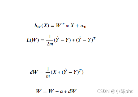
梯度求导公式

对应的梯度计算，a 代表学习率

class MultivariateNetwork():
    def __init__(self, num_of_features=1, learning_rate=0.1):
        """
        This function creates a vector of zeros of shape (num_of_features, 1) for W and initializes w_0 to 0.

        Argument:
        num_of_features -- size of the W vector, i.e., the number of features, excluding the bias

        Returns:
        W -- initialized vector of shape (dim, 1)
        w_0 -- initialized scalar (corresponds to the bias)
        """
        # n is the number of features
        self.n = num_of_features
        # alpha is the learning rate
        self.alpha = learning_rate

        ### START YOUR CODE HERE ###
        # initialize self.W and self.w_0 to be 0's
        self.W = np.zeros((self.n, 1))
        self.w_0 = 0
        ### YOUR CODE ENDS ###
        assert (self.W.shape == (self.n, 1))
        assert (isinstance(self.w_0, float) or isinstance(self.w_0, int))

    def fit(self, X, Y, epochs=1000, print_loss=True):
        """
        This function implements the Gradient Descent Algorithm
        Arguments:
        X -- training data matrix: each column is a training example.
                The number of columns is equal to the number of training examples
        Y -- true "label" vector: shape (1, m)
        epochs --

        Return:
        params -- dictionary containing weights
        losses -- loss values of every 100 epochs
        grads -- dictionary containing dW and dw_0
        """
        losses = []

        for i in range(epochs):
            # Get the number of training examples
            m = X.shape[1]

            ### START YOUR CODE HERE ###
            # Calculate the hypothesis outputs Y_hat (≈ 1 line of code)
            # (n,m)@(m,1) = (n,m)
            # print(X.shape)
            # print(self.W.shape)


            Y_hat = X.T @ self.W + self.w_0
            Y = Y.reshape(-1,1)




            # Calculate loss (≈ 1 line of code)

            loss =( 1 / (2 * m) * (Y - Y_hat)*(Y - Y_hat)).sum().mean()

            # print(loss)
            # exit()
            # Calculate the gredients for W and w_0
            dW = 1 / m * (X @ (Y - Y_hat))

            # print(dW)
            dw_0 = np.sum(1 / m * (Y - Y_hat))

            # Weight updates
            self.W = self.W + self.alpha * dW
            self.w_0 = self.w_0 + self.alpha * dw_0
            ### YOUR CODE ENDS ###

            if ((i % 100) == 0):
                losses.append(loss)
                # Print the cost every 100 training examples
                if print_loss:
                    print("Cost after iteration %i: %f" % (i, loss))

        params = {
            "W": self.W,
            "w_0": self.w_0
        }

        grads = {
            "dw":dW,
            "dw_0": dw_0
        }

        return params, grads, losses


    def predict(self, X):
        '''
        Predict the actual values using learned parameters (self.W, self.w_0)

        Arguments:
        X -- data of size (n x m)

        Returns:
        Y_prediction -- a numpy array (vector) containing all predictions for the examples in X
        '''
        m = X.shape[1]
        Y_prediction = np.zeros((1, m))

        # Compute the actual values
        ### START YOUR CODE HERE ###
        # (n,m)@(m,1) + b ===>(n,1)
        Y_prediction = X.T@self.W+self.w_0
        ### YOUR CODE ENDS ###

        return Y_prediction

    def normalize(self, matrix):
        '''
        matrix: the matrix that needs to be normalized. Note that each column represents a training example.
             The number of columns is the the number of training examples
        '''
        # (n,m)
        # Calculate mean for each feature
        # Pay attention to the value of axis = ?
        # set keepdims=True to avoid rank-1 array
        ### START YOUR CODE HERE ###
        # calculate mean (1 line of code)
        mean =np.mean(matrix,axis=0,keepdims=True)
        # calculate standard deviation (1 line of code)
        std = np.std(matrix,axis=0,keepdims=True)
        # normalize the matrix based on mean and std
        matrix = (matrix-mean)/std
        ### YOUR CODE ENDS ###
        return matrix

训练代码

def Run_Experiment(X_train, Y_train, X_test, Y_test, epochs=2000, learning_rate=0.5, print_loss=False):
    """
    Builds the multivariate linear regression model by calling the function you've implemented previously

    Arguments:
    X_train -- training set represented by a numpy array
    Y_train -- training labels represented by a numpy array (vector)
    X_test -- test set represented by a numpy array
    Y_test -- test labels represented by a numpy array (vector)
    epochs -- hyperparameter representing the number of iterations to optimize the parameters
    learning_rate -- hyperparameter representing the learning rate used in the update rule of optimize()
    print_loss -- Set to true to print the cost every 100 iterations

    Returns:
    d -- dictionary containing information about the model.
    """
    num_of_features = X_train.shape[0]
    model = MultivariateNetwork(num_of_features, learning_rate)

    ### START YOUR CODE HERE ###
    # Obtain the parameters, gredients, and losses by calling a model's method (≈ 1 line of code)
    # print(X_train)
    # exit()
    # print(X_train[:1])
    # X_train = model.normalize(matrix=X_train[:1])
    # print(X_train)
    # exit()


    parameters, grads, losses = model.fit(X_train,Y_train,epochs=epochs)

    # Predict test/train set examples (≈ 2 lines of code)
    Y_prediction_test =model.predict(X_test)
    Y_prediction_train = model.predict(X_train)
    ### YOUR CODE ENDS ###

    # Print train/test Errors
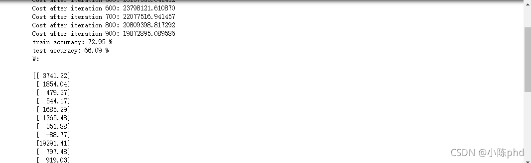
    print("train accuracy: {:.2f} %".format(abs(100 - np.mean(np.abs(Y_prediction_train - Y_train) / Y_train) * 100)))
    print("test accuracy: {:.2f} %".format(abs(100 - np.mean(np.abs(Y_prediction_test - Y_test) / Y_test) * 100)))

    np.set_printoptions(precision=2)
    W = parameters['W']
    w_0 = parameters['w_0']
    print("W: \n")
    print(W)
    print("w_0: {:.2f}".format(w_0))
    print(w_0)

    d = {"losses": losses,
         "Y_prediction_test": Y_prediction_test,
         "Y_prediction_train": Y_prediction_train,
         "W": W,
         "w_0": w_0,
         "learning_rate": learning_rate,
         "epochs": epochs}

    return d

实战 ，拿个训练集试一下

df = pd.read_csv('prj2data1.csv', header=None)
X_train = df[[0, 1]].values.T
Y_train = df[2].values.reshape(-1, 1).T


df_test = pd.read_csv('prj2data1_test.csv', header=None)
X_test = df_test[[0, 1]].values.T
Y_test = df_test[2].values.reshape(-1, 1).T
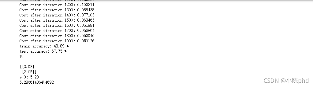
d = Run_Experiment(X_train, Y_train, X_test, Y_test, epochs = 2000, learning_rate = 0.01, print_loss = True)

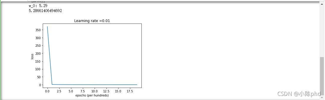
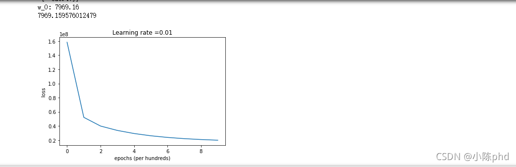
# Plot learning curve (with costs)
losses = np.squeeze(d['losses'])
plt.plot(losses)
plt.ylabel('loss')
plt.xlabel('epochs (per hundreds)')
plt.title("Learning rate =" + str(d["learning_rate"]))
plt.show()

之后会的到损失显示，对应参数的显示，以及损失曲线

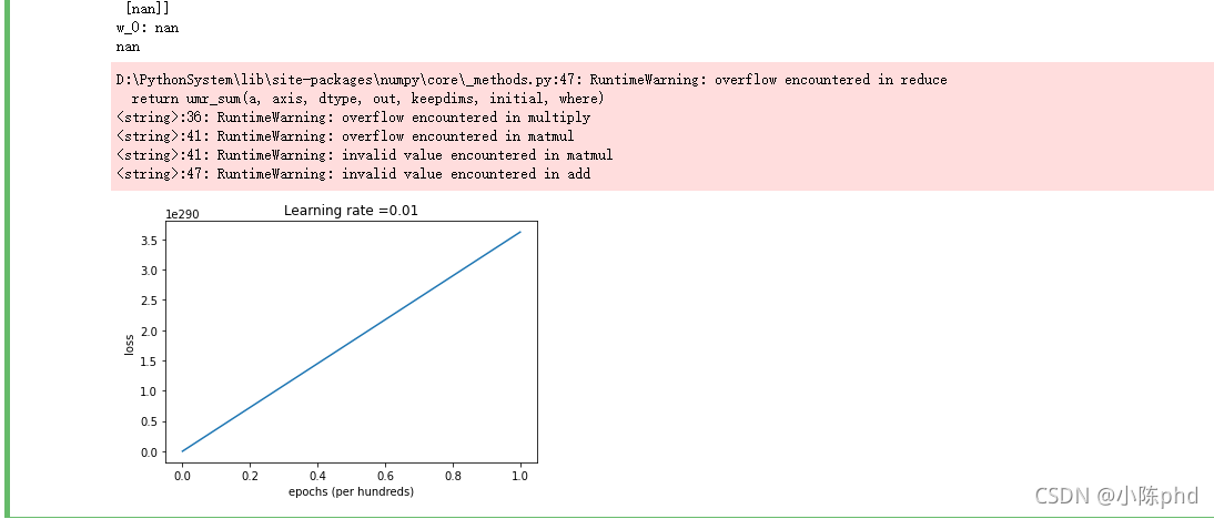
不对标签进行标准化,结果

• 发现有些特征差异太大，在进行求导时，会导致梯度爆炸

# Prepare Train/Test data
df = pd.read_csv('encoded_insurance.csv', header=None, skiprows=1)

train_test_ratio = 0.7
range_train = int(len(df) * train_test_ratio)
X_train = df.iloc[:range_train, :-1]
Y_train = df.iloc[:range_train, -1]
X_test = df.iloc[range_train:, :-1]
Y_test = df.iloc[range_train:, -1]

X_train = X_train.values.T
Y_train = Y_train.values.reshape(1, -1)
X_test = X_test.values.T
Y_test = Y_test.values.reshape(1, -1)
d = Run_Experiment(X_train, Y_train, X_test, Y_test, epochs = 1000, learning_rate = 0.01, print_loss = True)
# Plot learning curve (with costs)
losses = np.squeeze(d['losses'])
plt.plot(losses)
plt.ylabel('loss')
plt.xlabel('epochs (per hundreds)')
plt.title("Learning rate =" + str(d["learning_rate"]))
plt.show()

对数据进行标准化

model2 = MultivariateNetwork()
# print(X_train[0].shape)
X_train[0] = model2.normalize(X_train[0])
X_train[1] = model2.normalize(X_train[1])
X_test[0] = model2.normalize(X_test[0])
X_test[1] = model2.normalize(X_test[1])


# print(X_train)
d = Run_Experiment(X_train, Y_train, X_test, Y_test, epochs = 1000, learning_rate = 0.01, print_loss = True)
# Plot learning curve (with costs)
losses = np.squeeze(d['losses'])
plt.plot(losses)
plt.ylabel('loss')
plt.xlabel('epochs (per hundreds)')
plt.title("Learning rate =" + str(d["learning_rate"]))
plt.show()

发现效果不是很好，考虑对价格(因变量)进行分析

fig= plt.figure(figsize=(12,4))

ax=fig.add_subplot(111)
sns.distplot(df.iloc[:, -1],bins=50,color='r',ax=ax)
ax.set_title('Distribution of insurance charges')

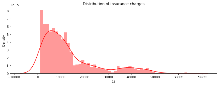
• 让我们分析因变量的特征。 由此可见，因变量“电荷”是不正常的。 然而，正态性在统计学和线性回归中非常重要。

fig= plt.figure(figsize=(12,4))

ax=fig.add_subplot(111)
#Pay attention to the log
sns.distplot(np.log(df.iloc[:,-1]),bins=40,color='b',ax=ax)
ax.set_title('Distribution of insurance charges in $log$ sacle')
ax.set_xscale('log');

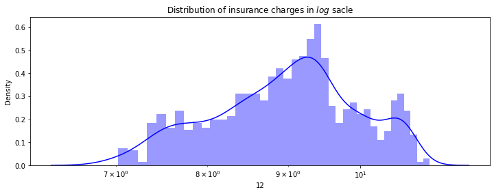
因此对标签进行对数变换

### START YOUR CODE HERE ###
#Normalize dependent variable using logarithm transformation
Y_train = np.log(1+Y_train)
Y_test = np.log(1+Y_test)
### YOUR CODE ENDS ###

d = Run_Experiment(X_train, Y_train, X_test, Y_test, epochs = 1000, learning_rate = 0.01, print_loss = True)
# Plot learning curve (with costs)
losses = np.squeeze(d['losses'])
plt.plot(losses)
plt.ylabel('loss')
plt.xlabel('epochs (per hundreds)')
plt.title("Learning rate =" + str(d["learning_rate"]))
plt.show()

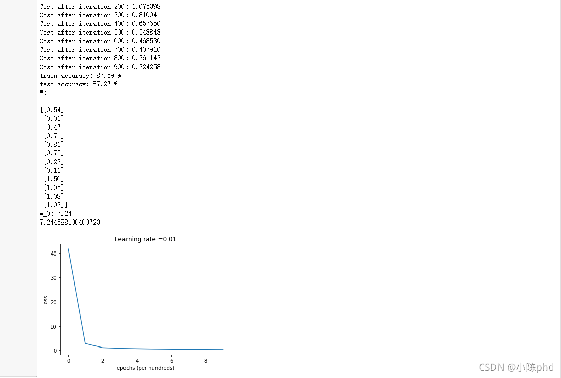
• 训练得分，测试得分明显改善