一.用Excel中数据分析功能做线性回归
1.取20组数据
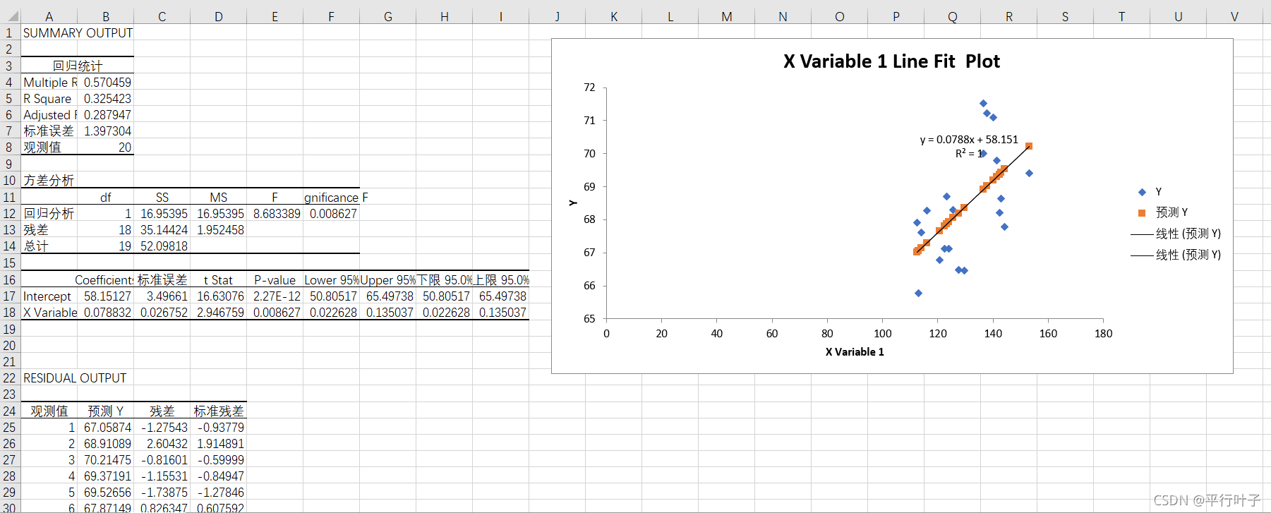
得出线性回归方程为y=0.0788x+58.151,相关系数R2为0.570459。
2.取200组数据
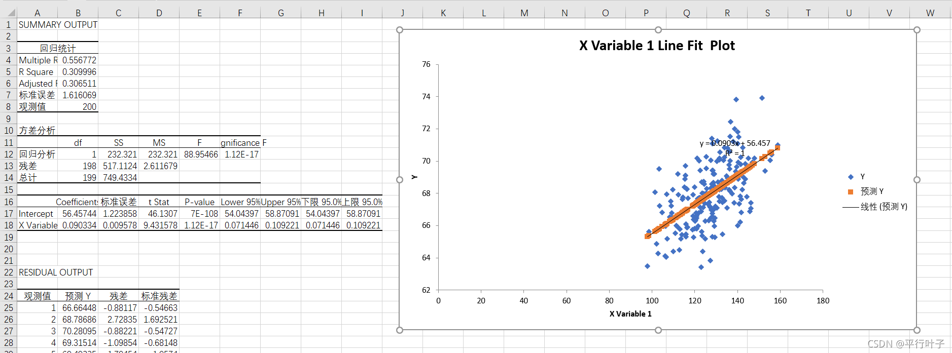
得出线性回归方程为y=0.0903x+56.457,相关系数R2为0.556772。
3.取2000组数据
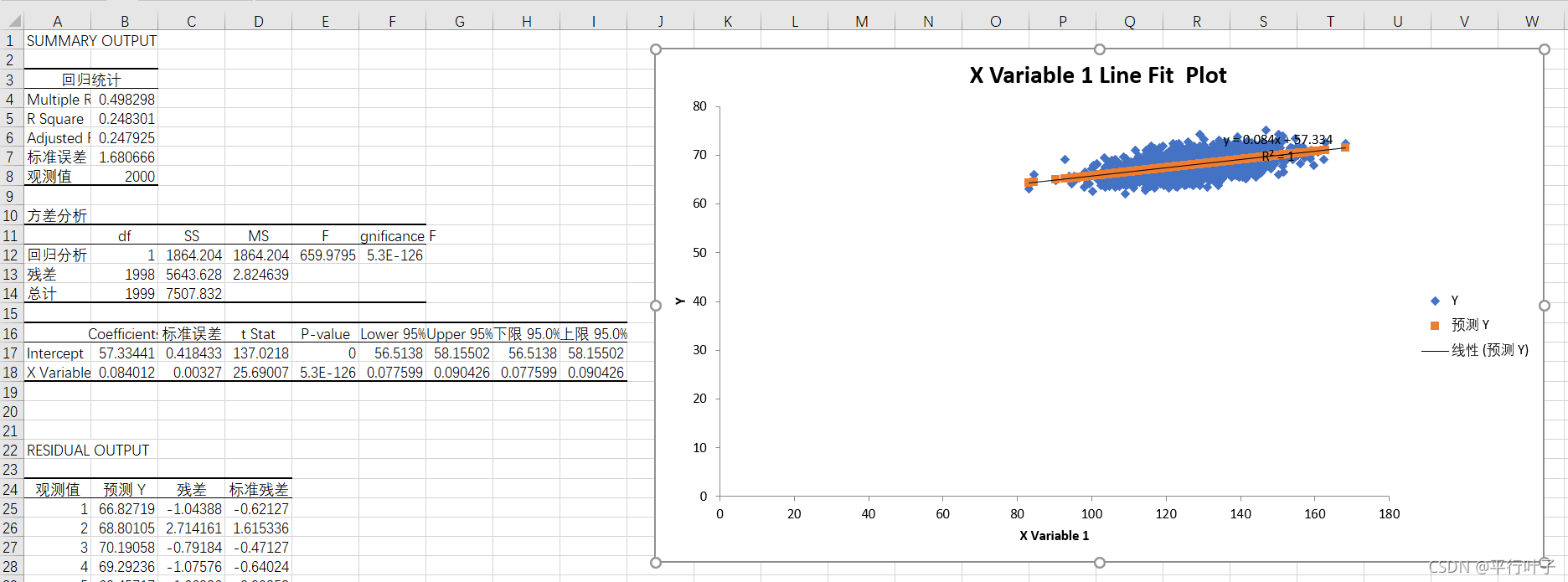
得出线性回归方程为y=0.084x+57.334,相关系数R2为0.498298。
二.用jupyter编程(不借助第三方库),用最小二乘法做线性回归
python最小二乘法源代码
import numpy as np
import matplotlib.pyplot as plt
%matplotlib inline
points = np.genfromtxt("D:/wh.csv",delimiter=",")
#将wh.csv文件中的数据赋值给points
#将points中的数据分别赋给x,y,求回归方程y=ax+b
x=points[0:20,1];
y=points[0:20,0];
#根据自己需要使用数据的个数更改[]中的值
pccs = np.corrcoef(x, y)
c,d=pccs
e,f=c
x_mean = np.mean(x)
y_mean = np.mean(y)
xsize = x.size
zi = (x * y).sum() - xsize * x_mean *y_mean
mu = (x ** 2).sum() - xsize * x_mean ** 2
a = zi / mu
b = y_mean - a * x_mean
a = np.around(a,decimals=2)
b = np.around(b,decimals=2)
print(f'回归线方程:y = {a}x + {b}')
print(f'相关系数为{f}')
#使用第三方库skleran画出拟合曲线
y1 = a*x + b
plt.scatter(x,y)
plt.plot(x,y1,c='r')
1.取20组数据
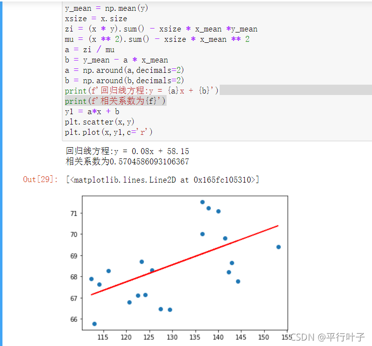
得出线性回归方程为y=0.08x+58.15,相关系数R2为0.5704。
2.取200组数据
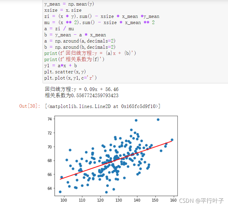
得出线性回归方程为y=0.09x+56.46,相关系数R2为0.5567。
3.取2000组数据
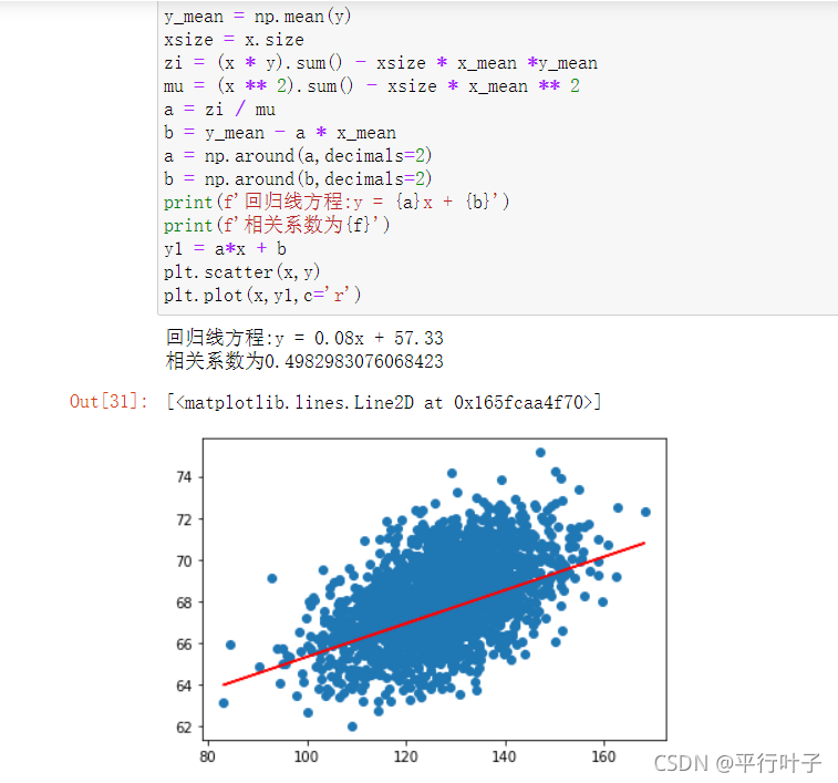
得出线性回归方程为y=0.08x+57.33,相关系数R2为0.4982。
三.用jupyter编程,借助skleran做线性回归
python借助skleran源代码
from sklearn import linear_model        #表示,可以调用sklearn中的linear_model模块进行线性回归。
import matplotlib.pyplot as plt
import numpy as np
%matplotlib inline
data = np.loadtxt(open("D:wh.csv","rb"),delimiter=",",skiprows=0)
data1=data[0:20]#根据所取数据更改值
x=[example[1] for example in data1]
y=[example[0] for example in data1]
pccs = np.corrcoef(x, y)
c,d=pccs
e,f=c
X = np.asarray(x).reshape(-1, 1)
Y = np.asarray(y).reshape(-1, 1)
model = linear_model.LinearRegression()
model.fit(X,Y)
b=model.intercept_[0] #截距
a=model.coef_[0]#线性模型的系数
a1=a[0]
print(f'回归线方程:y = {a1}x + {b}')
print(f'相关系数为{f}')
y1 = a1*X + b
plt.scatter(X,Y)
plt.plot(x,y1,c='r')
1.取20组数据
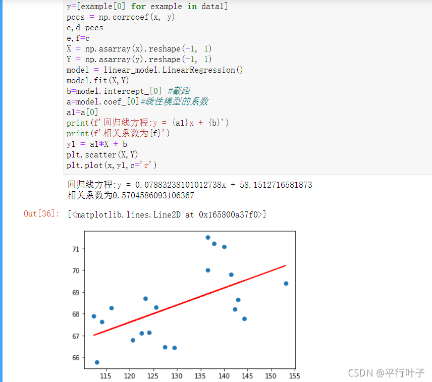
得出线性回归方程为y = 0.0788x + 58.1512,相关系数R2为0.5704。
2.取200组数据
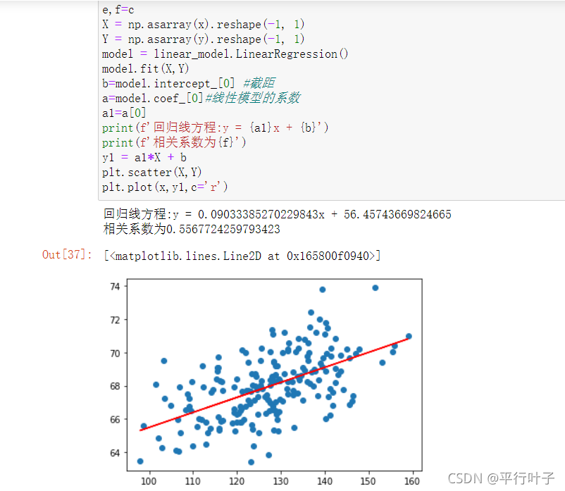
得出线性回归方程为y = 0.0903x + 56.4574,相关系数R2为0.5567。
3.取2000组数据
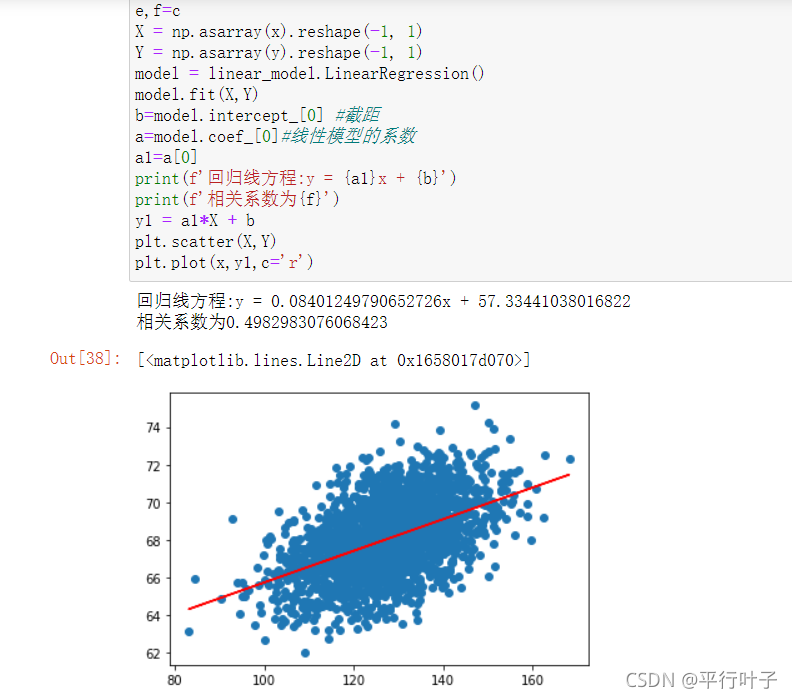
得出线性回归方程为y = 0.0840x + 57.3344,相关系数R2为0.4982。
四.总结
三种求线性回归方程的方法求出的值基本一致,但利用编程计算时,当数据的个数改变时,只需要改变代码中某个值就能快速得出线性回归方程,这比仅使用Excel更快速方便,特别是调用第三方库时,更加方便。