һ��MobileNetV1 ����
��Ҫ�Ķ��ȸ�2017������ġ�MobileNets: Efficient Convolutional Neural Networks for Mobile Vision Applications��,��� Depthwise ���� �� Pointwise ������ͬʱ,�Ķ�����:https://github.com/OUCTheoryGroup/colab_demo/blob/master/202003_models/MobileNetV1_CIFAR10.ipynb �Ѵ������� Colab ����,�۲첢���Ч����
BatchNorm2d()?:��ʹ��pytorch�� nn.BatchNorm2d() ���ʱ��,������ʹ�÷�ʽΪ�ڲ�������ֻ���ϴ����������ݵ�ͨ����(��������)�������Ǹ���ͳ�Ƶ�mean ��var�������ݽ��б���,�������mena��var��ÿ��batch(����һ��cost��Ҫ�������������,�����ݼ��Ƚϴ��ʱ��,һ���Խ�������������ȥ����һ��cost�洢��Բ���,��˻����һ������һ����������������ѵ����)�ж�����С�
Depthwise ����һ����ͨ����ͼ��,ʹ��3��3�ľ�����,��ȫ�ڶ�άƽ���Ͻ���,�����˵������������ͨ������ͬ,���Ծ������������3��feature map�������IJ���Ϊ: 3 �� 3 �� 3 = 27,������ʾ:
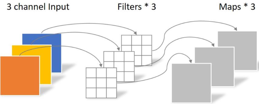
Pointwise ��֮ͬ�����ھ����˵ijߴ�Ϊ1��1��k,kΪ����ͨ��������������,����ľ�������Ὣ��һ���feature map��Ȩ�ں�,�м���filter���м���feature map,��������Ϊ:1 �� 1 �� 3 �� 4 = 12,����ͼ��ʾ:
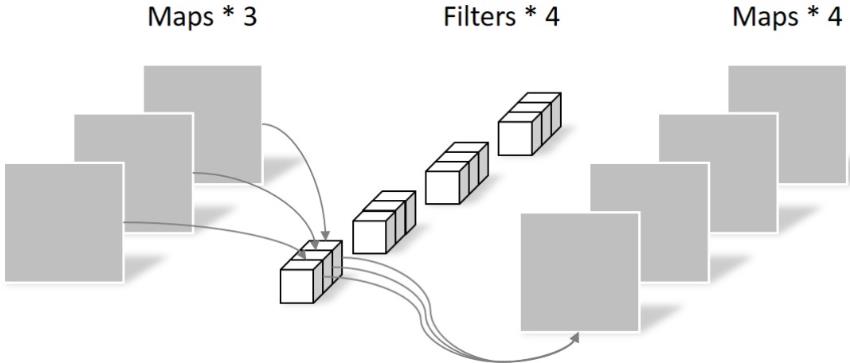
?���,���Կ���,ͬ���õ�4��feature map,ʹ��Depthwise+Pointwise����,�����������Դ�͡�
���벿��
?MobileNet �ɷ������
import torch
import torch.nn as nn
import torch.nn.functional as F
import torchvision
import torchvision.transforms as transforms
import matplotlib.pyplot as plt
import numpy as np
import torch.optim as optim
class Block(nn.Module):
'''Depthwise conv + Pointwise conv'''
def __init__(self, in_planes, out_planes, stride=1):
super(Block, self).__init__()
# Depthwise ����,3*3 �ľ�����,��Ϊ in_planes,�����㵥�����о���
self.conv1 = nn.Conv2d(in_planes, in_planes, kernel_size=3, stride=stride, padding=1, groups=in_planes, bias=False)
self.bn1 = nn.BatchNorm2d(in_planes)
# Pointwise ����,1*1 �ľ�����
self.conv2 = nn.Conv2d(in_planes, out_planes, kernel_size=1, stride=1, padding=0, bias=False)
self.bn2 = nn.BatchNorm2d(out_planes)
def forward(self, x):
out = F.relu(self.bn1(self.conv1(x)))
out = F.relu(self.bn2(self.conv2(out)))
return out?���� DataLoader
# ʹ��GPUѵ��,�����ڲ˵� "����ִ�й���" -> "��������ʱ����" ���������
device = torch.device("cuda:0" if torch.cuda.is_available() else "cpu")
transform_train = transforms.Compose([
transforms.RandomCrop(32, padding=4),
transforms.RandomHorizontalFlip(),
transforms.ToTensor(),
transforms.Normalize((0.4914, 0.4822, 0.4465), (0.2023, 0.1994, 0.2010))])
transform_test = transforms.Compose([
transforms.ToTensor(),
transforms.Normalize((0.4914, 0.4822, 0.4465), (0.2023, 0.1994, 0.2010))])
trainset = torchvision.datasets.CIFAR10(root='./data', train=True, download=True, transform=transform_train)
testset = torchvision.datasets.CIFAR10(root='./data', train=False, download=True, transform=transform_test)
trainloader = torch.utils.data.DataLoader(trainset, batch_size=128, shuffle=True, num_workers=2)
testloader = torch.utils.data.DataLoader(testset, batch_size=128, shuffle=False, num_workers=2)���� MobileNetV1 ����
32��32��3 ==>
32��32��32 ==> 32��32��64 ==> 16��16��128 ==> 16��16��128 ==>
8��8��256 ==> 8��8��256 ==> 4��4��512 ==> 4��4��512 ==>
2��2��1024 ==> 2��2��1024
������Ϊ��ֵ pooling ==> 1��1��1024
���ȫ���ӵ� 10������ڵ�
class MobileNetV1(nn.Module):
    # (128,2) means conv planes=128, stride=2
    cfg = [(64,1), (128,2), (128,1), (256,2), (256,1), (512,2), (512,1),
           (1024,2), (1024,1)]

    def __init__(self, num_classes=10):
        super(MobileNetV1, self).__init__()
        self.conv1 = nn.Conv2d(3, 32, kernel_size=3, stride=1, padding=1, bias=False)
        self.bn1 = nn.BatchNorm2d(32)
        self.layers = self._make_layers(in_planes=32)
        self.linear = nn.Linear(1024, num_classes)

    def _make_layers(self, in_planes):
        layers = []
        for x in self.cfg:
            out_planes = x[0]
            stride = x[1]
            layers.append(Block(in_planes, out_planes, stride))
            in_planes = out_planes
        return nn.Sequential(*layers)

    def forward(self, x):
        out = F.relu(self.bn1(self.conv1(x)))
        out = self.layers(out)
        out = F.avg_pool2d(out, 2)
        out = out.view(out.size(0), -1)
        out = self.linear(out)
return outʵ��������
# ����ŵ�GPU��
net = MobileNetV1().to(device)
criterion = nn.CrossEntropyLoss()
optimizer = optim.Adam(net.parameters(), lr=0.001)ģ��ѵ��
for epoch in range(10): # �ظ�����ѵ��
for i, (inputs, labels) in enumerate(trainloader):
inputs = inputs.to(device)
labels = labels.to(device)
# �Ż����ݶȹ���
optimizer.zero_grad()
# ���� +������ + �Ż�
outputs = net(inputs)
loss = criterion(outputs, labels)
loss.backward()
optimizer.step()
# ���ͳ����Ϣ
if i % 100 == 0:
print('Epoch: %d Minibatch: %5d loss: %.3f' %(epoch + 1, i + 1, loss.item()))
print('Finished Training')
ģ�Ͳ���?
correct = 0
total = 0

for data in testloader:
    images, labels = data
    images, labels = images.to(device), labels.to(device)
    outputs = net(images)
    _, predicted = torch.max(outputs.data, 1)
    total += labels.size(0)
    correct += (predicted == labels).sum().item()

print('Accuracy of the network on the 10000 test images: %.2f %%' % (
100 * correct / total))����MobileNetV2 ����
��Ҫ�Ķ��ȸ���CVPR2018�ϵ����ġ�MobileNetV2: Inverted Residuals and Linear Bottlenecks��,���ڶ����汾�ĸĽ����Ķ�����:https://github.com/OUCTheoryGroup/colab_demo/blob/master/202003_models/MobileNetV2_CIFAR10.ipynb �Ѵ������� Colab ����,�۲첢���Ч����
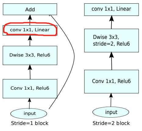
MobileNet V2 ����Ҫ�Ķ�һ:�����Inverted residual block
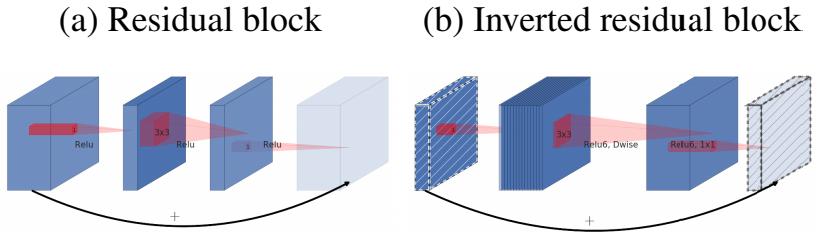
ResNet�е�bottleneck,����1x1������ͨ������256����64,Ȼ�����3x3����,��Ȼ�м�3x3����������̫������bottleneck�����߿��м�խ(Ҳ�����ֵ�����)��
���������м��3x3�������Ա��Depthwise,������������,����ͨ�����Զ�һЩ������MobileNet V2 ����1x1��������ͨ����,Ȼ����Depthwise 3x3�ľ���,��ʹ��1x1�ľ�����ά�����߳�֮ΪInverted residual block,�м������խ��
MobileNet V2 ����Ҫ�Ķ���:ȥ��������ֵ�ReLU6
�� MobileNet V1 ����ʹ�� ReLU6,ReLU6 ������ͨ��ReLU��������������ֵΪ 6,����Ϊ�����ƶ����豸 float16/int8 �ĵ;��ȵ�ʱ��,Ҳ���кܺõ���ֵ�ֱ��ʡ�Depthwise����Ƚ�dz,Ӧ��ReLU�������Ϣ��ʧ,����������ReLUȥ����(ע����ͼ�б��IJ���û��ReLU)��
?���벿��
import torch
import torch.nn as nn
import torch.nn.functional as F
import torchvision
import torchvision.transforms as transforms
import matplotlib.pyplot as plt
import numpy as np
import torch.optim as optim
class Block(nn.Module):
'''expand + depthwise + pointwise'''
def __init__(self, in_planes, out_planes, expansion, stride):
super(Block, self).__init__()
self.stride = stride
# ͨ�� expansion ���� feature map ������
planes = expansion * in_planes
self.conv1 = nn.Conv2d(in_planes, planes, kernel_size=1, stride=1, padding=0, bias=False)
self.bn1 = nn.BatchNorm2d(planes)
self.conv2 = nn.Conv2d(planes, planes, kernel_size=3, stride=stride, padding=1, groups=planes, bias=False)
self.bn2 = nn.BatchNorm2d(planes)
self.conv3 = nn.Conv2d(planes, out_planes, kernel_size=1, stride=1, padding=0, bias=False)
self.bn3 = nn.BatchNorm2d(out_planes)
# ����Ϊ 1 ʱ,��� in �� out �� feature map ͨ����ͬ,��һ�������ı�ͨ����
if stride == 1 and in_planes != out_planes:
self.shortcut = nn.Sequential(
nn.Conv2d(in_planes, out_planes, kernel_size=1, stride=1, padding=0, bias=False),
nn.BatchNorm2d(out_planes))
# ����Ϊ 1 ʱ,��� in �� out �� feature map ͨ����ͬ,ֱ�ӷ�������
if stride == 1 and in_planes == out_planes:
self.shortcut = nn.Sequential()
def forward(self, x):
out = F.relu(self.bn1(self.conv1(x)))
out = F.relu(self.bn2(self.conv2(out)))
out = self.bn3(self.conv3(out))
# ����Ϊ1,�� shortcut ����
if self.stride == 1:
return out + self.shortcut(x)
# ����Ϊ2,ֱ�����
else:
return out���� MobileNetV2 ����
ע��,��Ϊ CIFAR10 �� 32*32,���,������һ���ġ�
class MobileNetV2(nn.Module):
    # (expansion, out_planes, num_blocks, stride)
    cfg = [(1,  16, 1, 1),
           (6,  24, 2, 1),
           (6,  32, 3, 2),
           (6,  64, 4, 2),
           (6,  96, 3, 1),
           (6, 160, 3, 2),
           (6, 320, 1, 1)]

    def __init__(self, num_classes=10):
        super(MobileNetV2, self).__init__()
        self.conv1 = nn.Conv2d(3, 32, kernel_size=3, stride=1, padding=1, bias=False)
        self.bn1 = nn.BatchNorm2d(32)
        self.layers = self._make_layers(in_planes=32)
        self.conv2 = nn.Conv2d(320, 1280, kernel_size=1, stride=1, padding=0, bias=False)
        self.bn2 = nn.BatchNorm2d(1280)
        self.linear = nn.Linear(1280, num_classes)

    def _make_layers(self, in_planes):
        layers = []
        for expansion, out_planes, num_blocks, stride in self.cfg:
            strides = [stride] + [1]*(num_blocks-1)
            for stride in strides:
                layers.append(Block(in_planes, out_planes, expansion, stride))
                in_planes = out_planes
        return nn.Sequential(*layers)

    def forward(self, x):
        out = F.relu(self.bn1(self.conv1(x)))
        out = self.layers(out)
        out = F.relu(self.bn2(self.conv2(out)))
        out = F.avg_pool2d(out, 4)
        out = out.view(out.size(0), -1)
        out = self.linear(out)
return out���� DataLoader
# ʹ��GPUѵ��,�����ڲ˵� "����ִ�й���" -> "��������ʱ����" ���������
device = torch.device("cuda:0" if torch.cuda.is_available() else "cpu")
transform_train = transforms.Compose([
transforms.RandomCrop(32, padding=4),
transforms.RandomHorizontalFlip(),
transforms.ToTensor(),
transforms.Normalize((0.4914, 0.4822, 0.4465), (0.2023, 0.1994, 0.2010))])
transform_test = transforms.Compose([
transforms.ToTensor(),
transforms.Normalize((0.4914, 0.4822, 0.4465), (0.2023, 0.1994, 0.2010))])
trainset = torchvision.datasets.CIFAR10(root='./data', train=True, download=True, transform=transform_train)
testset = torchvision.datasets.CIFAR10(root='./data', train=False, download=True, transform=transform_test)
trainloader = torch.utils.data.DataLoader(trainset, batch_size=128, shuffle=True, num_workers=2)
testloader = torch.utils.data.DataLoader(testset, batch_size=128, shuffle=False, num_workers=2)ʵ��������
# ����ŵ�GPU��
net = MobileNetV2().to(device)
criterion = nn.CrossEntropyLoss()
optimizer = optim.Adam(net.parameters(), lr=0.001)ģ��ѵ��
for epoch in range(10): # �ظ�����ѵ��
for i, (inputs, labels) in enumerate(trainloader):
inputs = inputs.to(device)
labels = labels.to(device)
# �Ż����ݶȹ���
optimizer.zero_grad()
# ���� +������ + �Ż�
outputs = net(inputs)
loss = criterion(outputs, labels)
loss.backward()
optimizer.step()
# ���ͳ����Ϣ
if i % 100 == 0:
print('Epoch: %d Minibatch: %5d loss: %.3f' %(epoch + 1, i + 1, loss.item()))
print('Finished Training')ģ�Ͳ���?
correct = 0
total = 0

for data in testloader:
    images, labels = data
    images, labels = images.to(device), labels.to(device)
    outputs = net(images)
    _, predicted = torch.max(outputs.data, 1)
    total += labels.size(0)
    correct += (predicted == labels).sum().item()

print('Accuracy of the network on the 10000 test images: %.2f %%' % (
100 * correct / total))����HybridSN �߹���������
�Ķ����ġ�HybridSN: Exploring 3-D�C2-DCNN Feature Hierarchy for Hyperspectral Image Classification��,˼��3D������2D�����������Ķ�����:https://github.com/OUCTheoryGroup/colab_demo/blob/master/202003_models/HybridSN_GRSL2020.ipynb �Ѵ������� Colab ����,���粿����Ҫ�Լ���ɡ�ѵ������,Ȼ�����Լ���,�ᷢ��ÿ�η���Ľ������һ��,��˼��Ϊʲô?ͬʱ,˼������,�����Ҫ��һ�������߹���ͼ��ķ�������,������θĽ�?
��ƪ���Ĺ�����һ�� ������� ����߹���ͼ���������,������ 3D����,Ȼ��ʹ�� 2D������

����������:
- conv1:(1, 30, 25, 25), 8�� 7x3x3 �ľ����� ==>(8, 24, 23, 23)
- conv2:(8, 24, 23, 23), 16�� 5x3x3 �ľ����� ==>(16, 20, 21, 21)
- conv3:(16, 20, 21, 21),32�� 3x3x3 �ľ����� ==>(32, 18, 19, 19)
������Ҫ���ж�ά����,��˰�ǰ��� 32*18 reshape һ��,�õ� (576, 19, 19)
��ά����:(576, 19, 19) 64�� 3x3 �ľ�����,�õ� (64, 17, 17)
��������һ�� flatten ����,��Ϊ 18496 ά������,
����������Ϊ256,128�ڵ��ȫ���Ӳ�,��ʹ�ñ���Ϊ0.4�� Dropout,
������Ϊ 16 ���ڵ�,�����յķ����������
?
���벿��?
����ȡ������,��������������⡣
! wget http://www.ehu.eus/ccwintco/uploads/6/67/Indian_pines_corrected.mat
! wget http://www.ehu.eus/ccwintco/uploads/c/c4/Indian_pines_gt.mat
! pip install spectral
import numpy as np
import matplotlib.pyplot as plt
import scipy.io as sio
from sklearn.decomposition import PCA
from sklearn.model_selection import train_test_split
from sklearn.metrics import confusion_matrix, accuracy_score, classification_report, cohen_kappa_score
import spectral
import torch
import torchvision
import torch.nn as nn
import torch.nn.functional as F
import torch.optim as optim���� HybridSN ��
class_num = 16
class HybridSN(nn.Module):
''' your code here '''
# �������,��������ṹ�Ƿ�ͨ
# x = torch.randn(1, 1, 30, 25, 25)
# net = HybridSN()
# y = net(x)
# print(y.shape)�������ݼ�
���ȶԸ߹�������ʵʩPCA��ά;Ȼ�� keras ���㴦�������ݸ�ʽ;Ȼ�������ȡ 10% ������Ϊѵ����,ʣ�����Ϊ���Լ���
���ȶ����������:
# �Ը߹������� X Ӧ�� PCA �任
def applyPCA(X, numComponents):
newX = np.reshape(X, (-1, X.shape[2]))
pca = PCA(n_components=numComponents, whiten=True)
newX = pca.fit_transform(newX)
newX = np.reshape(newX, (X.shape[0], X.shape[1], numComponents))
return newX
# �Ե���������Χ��ȡ patch ʱ,��Ե���ؾ���ȡ��,���,���ⲿ�����ؽ��� padding ����
def padWithZeros(X, margin=2):
newX = np.zeros((X.shape[0] + 2 * margin, X.shape[1] + 2* margin, X.shape[2]))
x_offset = margin
y_offset = margin
newX[x_offset:X.shape[0] + x_offset, y_offset:X.shape[1] + y_offset, :] = X
return newX
# ��ÿ��������Χ��ȡ patch ,Ȼ���ɷ��� keras �����ĸ�ʽ
def createImageCubes(X, y, windowSize=5, removeZeroLabels = True):
# �� X �� padding
margin = int((windowSize - 1) / 2)
zeroPaddedX = padWithZeros(X, margin=margin)
# split patches
patchesData = np.zeros((X.shape[0] * X.shape[1], windowSize, windowSize, X.shape[2]))
patchesLabels = np.zeros((X.shape[0] * X.shape[1]))
patchIndex = 0
for r in range(margin, zeroPaddedX.shape[0] - margin):
for c in range(margin, zeroPaddedX.shape[1] - margin):
patch = zeroPaddedX[r - margin:r + margin + 1, c - margin:c + margin + 1]
patchesData[patchIndex, :, :, :] = patch
patchesLabels[patchIndex] = y[r-margin, c-margin]
patchIndex = patchIndex + 1
if removeZeroLabels:
patchesData = patchesData[patchesLabels>0,:,:,:]
patchesLabels = patchesLabels[patchesLabels>0]
patchesLabels -= 1
return patchesData, patchesLabels
def splitTrainTestSet(X, y, testRatio, randomState=345):
X_train, X_test, y_train, y_test = train_test_split(X, y, test_size=testRatio, random_state=randomState, stratify=y)
return X_train, X_test, y_train, y_test��ȡ���������ݼ�:
# �������
class_num = 16
X = sio.loadmat('Indian_pines_corrected.mat')['indian_pines_corrected']
y = sio.loadmat('Indian_pines_gt.mat')['indian_pines_gt']
# ���ڲ��������ı���
test_ratio = 0.90
# ÿ��������Χ��ȡ patch �ijߴ�
patch_size = 25
# ʹ�� PCA ��ά,�õ����ɷֵ�����
pca_components = 30
print('Hyperspectral data shape: ', X.shape)
print('Label shape: ', y.shape)
print('\n... ... PCA tranformation ... ...')
X_pca = applyPCA(X, numComponents=pca_components)
print('Data shape after PCA: ', X_pca.shape)
print('\n... ... create data cubes ... ...')
X_pca, y = createImageCubes(X_pca, y, windowSize=patch_size)
print('Data cube X shape: ', X_pca.shape)
print('Data cube y shape: ', y.shape)
print('\n... ... create train & test data ... ...')
Xtrain, Xtest, ytrain, ytest = splitTrainTestSet(X_pca, y, test_ratio)
print('Xtrain shape: ', Xtrain.shape)
print('Xtest shape: ', Xtest.shape)
# �ı� Xtrain, Ytrain ����״,�Է��� keras ��Ҫ��
Xtrain = Xtrain.reshape(-1, patch_size, patch_size, pca_components, 1)
Xtest = Xtest.reshape(-1, patch_size, patch_size, pca_components, 1)
print('before transpose: Xtrain shape: ', Xtrain.shape)
print('before transpose: Xtest shape: ', Xtest.shape)
# Ϊ����Ӧ pytorch �ṹ,����Ҫ�� transpose
Xtrain = Xtrain.transpose(0, 4, 3, 1, 2)
Xtest = Xtest.transpose(0, 4, 3, 1, 2)
print('after transpose: Xtrain shape: ', Xtrain.shape)
print('after transpose: Xtest shape: ', Xtest.shape)
""" Training dataset"""
class TrainDS(torch.utils.data.Dataset):
def __init__(self):
self.len = Xtrain.shape[0]
self.x_data = torch.FloatTensor(Xtrain)
self.y_data = torch.LongTensor(ytrain)
def __getitem__(self, index):
# ���������������ݺͶ�Ӧ�ı�ǩ
return self.x_data[index], self.y_data[index]
def __len__(self):
# �����ļ����ݵ���Ŀ
return self.len
""" Testing dataset"""
class TestDS(torch.utils.data.Dataset):
def __init__(self):
self.len = Xtest.shape[0]
self.x_data = torch.FloatTensor(Xtest)
self.y_data = torch.LongTensor(ytest)
def __getitem__(self, index):
# ���������������ݺͶ�Ӧ�ı�ǩ
return self.x_data[index], self.y_data[index]
def __len__(self):
# �����ļ����ݵ���Ŀ
return self.len
# ���� trainloader �� testloader
trainset = TrainDS()
testset = TestDS()
train_loader = torch.utils.data.DataLoader(dataset=trainset, batch_size=128, shuffle=True, num_workers=2)
test_loader = torch.utils.data.DataLoader(dataset=testset, batch_size=128, shuffle=False, num_workers=2)��ʼѵ��
# ʹ��GPUѵ��,�����ڲ˵� "����ִ�й���" -> "��������ʱ����" ���������
device = torch.device("cuda:0" if torch.cuda.is_available() else "cpu")
# ����ŵ�GPU��
net = HybridSN().to(device)
criterion = nn.CrossEntropyLoss()
optimizer = optim.Adam(net.parameters(), lr=0.001)
# ��ʼѵ��
total_loss = 0
for epoch in range(100):
for i, (inputs, labels) in enumerate(train_loader):
inputs = inputs.to(device)
labels = labels.to(device)
# �Ż����ݶȹ���
optimizer.zero_grad()
# ���� +������ + �Ż�
outputs = net(inputs)
loss = criterion(outputs, labels)
loss.backward()
optimizer.step()
total_loss += loss.item()
print('[Epoch: %d] [loss avg: %.4f] [current loss: %.4f]' %(epoch + 1, total_loss/(epoch+1), loss.item()))
print('Finished Training')ģ�Ͳ���
count = 0
# ģ�Ͳ���
for inputs, _ in test_loader:
inputs = inputs.to(device)
outputs = net(inputs)
outputs = np.argmax(outputs.detach().cpu().numpy(), axis=1)
if count == 0:
y_pred_test = outputs
count = 1
else:
y_pred_test = np.concatenate( (y_pred_test, outputs) )
# ���ɷ��౨��
classification = classification_report(ytest, y_pred_test, digits=4)
print(classification)���ú���
���������ڼ��������ȷ��,��ʾ����ı��ú���,�Թ��ο�
from operator import truediv
def AA_andEachClassAccuracy(confusion_matrix):
counter = confusion_matrix.shape[0]
list_diag = np.diag(confusion_matrix)
list_raw_sum = np.sum(confusion_matrix, axis=1)
each_acc = np.nan_to_num(truediv(list_diag, list_raw_sum))
average_acc = np.mean(each_acc)
return each_acc, average_acc
def reports (test_loader, y_test, name):
count = 0
# ģ�Ͳ���
for inputs, _ in test_loader:
inputs = inputs.to(device)
outputs = net(inputs)
outputs = np.argmax(outputs.detach().cpu().numpy(), axis=1)
if count == 0:
y_pred = outputs
count = 1
else:
y_pred = np.concatenate( (y_pred, outputs) )
if name == 'IP':
target_names = ['Alfalfa', 'Corn-notill', 'Corn-mintill', 'Corn'
,'Grass-pasture', 'Grass-trees', 'Grass-pasture-mowed',
'Hay-windrowed', 'Oats', 'Soybean-notill', 'Soybean-mintill',
'Soybean-clean', 'Wheat', 'Woods', 'Buildings-Grass-Trees-Drives',
'Stone-Steel-Towers']
elif name == 'SA':
target_names = ['Brocoli_green_weeds_1','Brocoli_green_weeds_2','Fallow','Fallow_rough_plow','Fallow_smooth',
'Stubble','Celery','Grapes_untrained','Soil_vinyard_develop','Corn_senesced_green_weeds',
'Lettuce_romaine_4wk','Lettuce_romaine_5wk','Lettuce_romaine_6wk','Lettuce_romaine_7wk',
'Vinyard_untrained','Vinyard_vertical_trellis']
elif name == 'PU':
target_names = ['Asphalt','Meadows','Gravel','Trees', 'Painted metal sheets','Bare Soil','Bitumen',
'Self-Blocking Bricks','Shadows']
classification = classification_report(y_test, y_pred, target_names=target_names)
oa = accuracy_score(y_test, y_pred)
confusion = confusion_matrix(y_test, y_pred)
each_acc, aa = AA_andEachClassAccuracy(confusion)
kappa = cohen_kappa_score(y_test, y_pred)
return classification, confusion, oa*100, each_acc*100, aa*100, kappa*100�����д���ļ���:
classification, confusion, oa, each_acc, aa, kappa = reports(test_loader, ytest, 'IP')
classification = str(classification)
confusion = str(confusion)
file_name = "classification_report.txt"

with open(file_name, 'w') as x_file:
    x_file.write('\n')
    x_file.write('{} Kappa accuracy (%)'.format(kappa))
    x_file.write('\n')
    x_file.write('{} Overall accuracy (%)'.format(oa))
    x_file.write('\n')
    x_file.write('{} Average accuracy (%)'.format(aa))
    x_file.write('\n')
    x_file.write('\n')
    x_file.write('{}'.format(classification))
    x_file.write('\n')
x_file.write('{}'.format(confusion))�������������ʾ������:
# load the original image
X = sio.loadmat('Indian_pines_corrected.mat')['indian_pines_corrected']
y = sio.loadmat('Indian_pines_gt.mat')['indian_pines_gt']
height = y.shape[0]
width = y.shape[1]
X = applyPCA(X, numComponents= pca_components)
X = padWithZeros(X, patch_size//2)
# ������Ԥ�����
outputs = np.zeros((height,width))
for i in range(height):
for j in range(width):
if int(y[i,j]) == 0:
continue
else :
image_patch = X[i:i+patch_size, j:j+patch_size, :]
image_patch = image_patch.reshape(1,image_patch.shape[0],image_patch.shape[1], image_patch.shape[2], 1)
X_test_image = torch.FloatTensor(image_patch.transpose(0, 4, 3, 1, 2)).to(device)
prediction = net(X_test_image)
prediction = np.argmax(prediction.detach().cpu().numpy(), axis=1)
outputs[i][j] = prediction+1
if i % 20 == 0:
print('... ... row ', i, ' handling ... ...')predict_image = spectral.imshow(classes = outputs.astype(int),figsize =(5,5))?