[È˹¤ÖÇÄÜ]The Robustness of Deep Networks A geometrical perspectiveÂÛÎĽâ¶Á

sciÂÛÎĵØÖ·

Introduction

Éñ¾­ÍøÂç½üЩÄêÒѾ­ÔÚÐí¶à³¡¾°Öеõ½ÁËÓ¦ÓÃ，µ«ÊÇһЩÉñ¾­ÍøÂçµÄ»ù´¡ÊôÐÔ»¹Ã»Óб»Àí½â，ÕâÒ²ÊǽüЩÄêÑо¿µÄÖص㡣¸ü¾ßÌåÀ´Ëµ，Éñ¾­ÍøÂç¶Ô¸÷ÖÖÀàÐÍperturbationµÄrobustnessÊܵ½Á˺ܴóµÄ¹Ø×¢¡£Í¼1²ûÊöÁËÉî¶ÈÉñ¾­ÍøÂç¶Ôsmall additive perturbationµÄ´àÈõÐÔ：

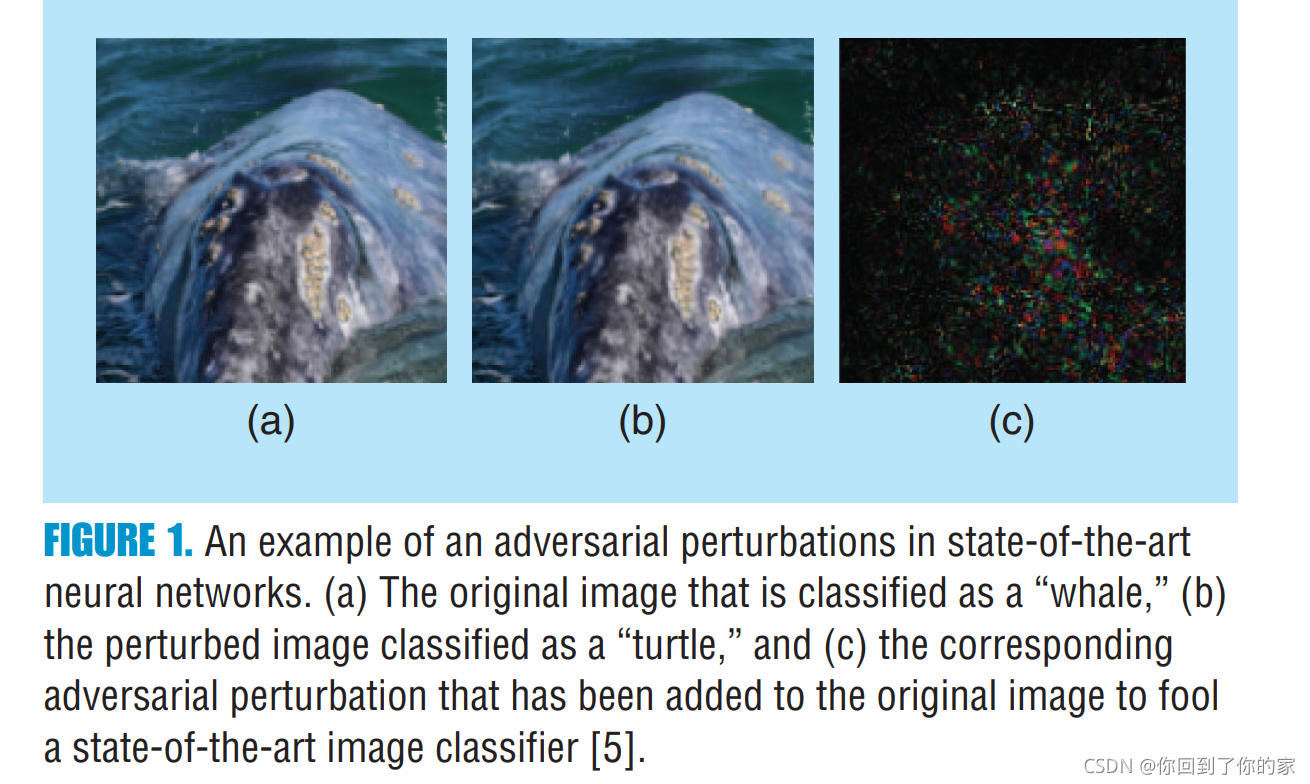
A dual phenomenon was observed in [3]，ÕâʱÈËÑÛÎÞ·¨Ê¶±ðµÄͼƬ»á±»Éî¶ÈÉñ¾­ÍøÂçÒԺܸߵÄconfidence½øÐзÖÀà¡£

The fundamental challenges raised by the robustness of deep networks to perturbationÒѾ­´ßÉú³öÁËÐí¶àÖØÒªµÄ¹¤×÷¡£ÕâЩ¹¤×÷´ÓʵÑéÉϺÍÀíÂÛÉ϶ÔÉî¶ÈÍøÂçÔÚ²»Í¬ÖÖÀàµÄperturbationÉϵÄrobustness½øÐÐÁËÑо¿，ÕâЩperturbation°üÀ¨adversarial perturbations，additive random noise，structured transformationsÉõÖÁuniversal perturbation¡£The robustness is usually measured as the sensitivity of the discrete classification function（¼´the function that assigns a label to each image）to such perturbation¡£¾¡¹Ü¶ÔÓÚrobustnessµÄ·ÖÎö²¢²»ÊÇÒ»¸öеÄÎÊÌâ，we provide an overview of the recent works that propose to assess the vulnerability of deep network architectures¡£³ýÁËÁ¿»¯ÔÚ¸÷ÖÖperturbationsÏÂÍøÂçµÄrobustness，¶ÔÓÚrobustnessµÄ·ÖÎöhas further contributed to developing important insights on the geometry of the complex decision boundary of such classifier， which remain hardly understood due to the very high dimensionality of the problems that they address¡£Êµ¼ÊÉÏ，Ò»¸ö·ÖÀàÆ÷µÄrobustnessÐÔÖʺ;ö²ß±ß½çµÄ¼¸ºÎÐÔÖÊÊǽôÃÜÏà¹ØµÄ¡£ÀýÈç，the high instability of Éî¶ÈÉñ¾­ÍøÂçto ¶Ô¿¹ÈŶ¯½Òʾ³öÊý¾Ýµãreside extremely close to the classifier¡®s decision boundary¡£¶ÔÓÚrobustnessµÄÑо¿Òò´Ë²»½öÄÜ°ïÖúÎÒÃÇ´Óʵ¼Ê½Ç¶ÈÀí½âϵͳµÄÎȶ¨ÐÔ，»¹ÄÜÔÊÐíÎÒÃÇÀí½â·ÖÀàÇøÓòµÄ¼¸ºÎÌØÕ÷²¢ÇÒʹµÃÎÒÃÇderives insight toward the improvement of current architectures¡£

ÕûƪÎÄÕÂÓжà¸öÄ¿µÄ¡£First, it provides an accessible review of the recent works in the analysis of the robustness of deep neural network classifiers to different forms of perturbations, with a particular emphasis on image analysis and visual understanding applications. Second, it presents connections between the robustness of deep networks and the geometry of the decision boundaries of such classifiers. Third, the article discusses ways to improve the robustness in deep networks architectures and finally highlights some of the important open problems.

Robustness of classifiers

ÔÚ´ó¶àÊýµÄ·ÖÀàÉ趨ÖÐ，²âÊÔÊý¾Ý¼¯ÖÐÎó·ÖÀàµÄ±ÈÀýÊÇÓÃÓÚÆÀ¼Û·ÖÀàÆ÷µÄÖ÷Òªperformance metric¡£The empirical test errorÌṩÁ˹ØÓÚ·ÖÀàÆ÷µÄrisk， defined as the probability of misclassification，when considering samples from the data distribution¡£ÕýʽÀ´½²，½« $¦Ì$ ¶¨ÒåΪa distribution defined over images¡£·ÖÀàÆ÷$f$µÄriskµÈ¼ÛÓÚ：

$$R(f)={\mathbb{P}}_{x¡«¦Ì}(f(x)ªÁ=y(x))(1)$$

$x$ºÍ$y(x)$·Ö±ð¶ÔÓ¦ÓÚͼƬºÍͼƬµÄlabel¡£While the risk captures the error of $f$ on the data distribution $¦Ì$，Ëü²¢Ã»Óв¶×½µ½the robustness to small arbitrary perturbations of data points¡£ÔÚÊÓ¾õ·ÖÀàÈÎÎñÖÐ，ÏÖÔÚÒ»¸ö±È½ÏÆÈÇеÄÈÎÎñÊÇѧϰµ½classifiers that achieve robustness to small perturbation to images¡£

ÕâÀﶨÒåһЩ·ûºÅ，ÈÃ$\mathcal{X}$±íʾthe ambient space where images live¡£ÈÃ$\mathcal{R}$±íʾÎÒÃÇËùÈÝÐíµÄÈŶ¯¼¯ºÏ¡£ÀýÈç，µ±¿¼ÂÇgeometric perturbationʱ，$\mathcal{R}$ is set to be the group of geometric（¼´ affine）transformation under study¡£Èç¹ûÎÒÃÇÏëÒªºâÁ¿ÔÚÈÎÒâadditive perturbationϵÄrobustness，ÄÇôÎÒÃÇÉ趨$\mathcal{R}=\mathcal{X}$¡£¶Ô$r¡Ê\mathcal{R}$，ÎÒÃǶ¨Òå$T_r:\mathcal{X}¡ú\mathcal{X}$to be the perturbation operator by $r$，¶ÔÓÚÒ»¸öÊý¾Ýµã$x¡Ê\mathcal{X}$，$T_r(x)$±íʾ±»$r$ÈŶ¯ºóµÄͼƬ$x$¡£Ê¹ÓÃÉÏÃæÕâЩnotations，ÎÒÃǽ«¸Ä±äÅбðÆ÷¹ØÓÚͼƬ$x$µÄlabelµÄ×îСperturbation¶¨ÒåΪ：

$$\begin{gathered} r^{?}(x)=\underset{r¡Ê\mathcal{R}}{\mathrm{argmin}}¡Îr{¡Î}_R \\ subjecttof(T_r(x))ªÁ=f(x)(2) \end{gathered}$$

ÕâÀï $¡Î?{¡Î}_R$ ÊÇ $\mathcal{R}$ ÉϵÄmetric¡£ÎªÁËnotation simplicity，ÎÒÃÇÊ¡ÂÔÁËthe dependence of $r^{?}(x)$ on $f$,$\mathcal{R}$,$¦Ä$and operator $T$¡£Moreover，µ±Í¼Æ¬$x$ is clear from the context，we will use $r^{?}$ to refer to $r^{?}(x)$¡£Í¼2¶ÔÈŶ¯¹ý³Ì½øÐÐÁ˲ûÊö：

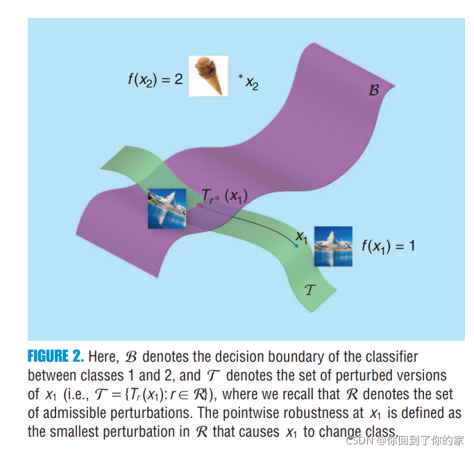
The pointwise robustness of $f$ at $x$ Òò´Ëͨ¹ý$¡Îr^{?}(x){¡Î}_{\mathcal{R}}$½øÐкâÁ¿¡£×¢Òâ$¡Î?{¡Î}_{\mathcal{R}}$ÖµÔ½´ó±íÃ÷$x$´¦µÄrobustnessÔ½¸ß¡£¾¡¹ÜÕâÖÖrobustnessµÄ¶¨Ò忼Âǵ½ÁËʹµÃ·ÖÀàÆ÷$f$¸Ä±ä·ÖÀàµÄ½á¹ûµÄsmallest perturbation $r^{?}(x)$，ÆäËûµÄ¹¤×÷È´²ÉÓÃÁËһЩÉÔ΢²»Í¬µÄ¶¨Òå，ÕâЩ¹¤×÷ÖÐa ¡®sufficiently small¡¯ perturbation is sought（instead of the minimal one）[7-9]¡£ÎªÁ˺âÁ¿·ÖÀàÆ÷$f$µÄglobal robustness，ÎÒÃÇ¿ÉÒÔ¼ÆËã$¡Îr^{?}(x){¡Î}_{\mathcal{R}}$ÔÚÊý¾Ý·Ö²¼ÉϵÄÆÚÍû¡£Õâ±íÃ÷global robustness $¦Ñ(f)$¿ÉÒÔͨ¹ýÈçϵķ½Ê½½øÐж¨Òå：

$$¦Ñ(f)={\mathbb{E}}_{x¡«¦Ì}(¡Îr^{?}(x){¡Î}_{\mathcal{R}}(3)$$

ÐèҪעÒâµÄ±È½ÏÖØÒªµÄÒ»µãÊÇ，ÔÚÎÒÃǵÄrobustness settingÖÐ，the perturbed point $T_r(x)$ need not belong to the support of the data distribution¡£Òò´Ë，¾¡¹Üthe focus of the risk in（1）is the accuracy on typical images（´Ó$¦Ì$ÖнøÐвÉÑù），the focus of the robustness computed from （2）is instead on the distance to the ¡®closest¡¯ image（potentially outside the support of $¦Ì$）that changes the label of the classifier¡£The risk and robustness hence capture two fundamentally different properties of the classifier，ÈçÈçÏÂËùÊö：

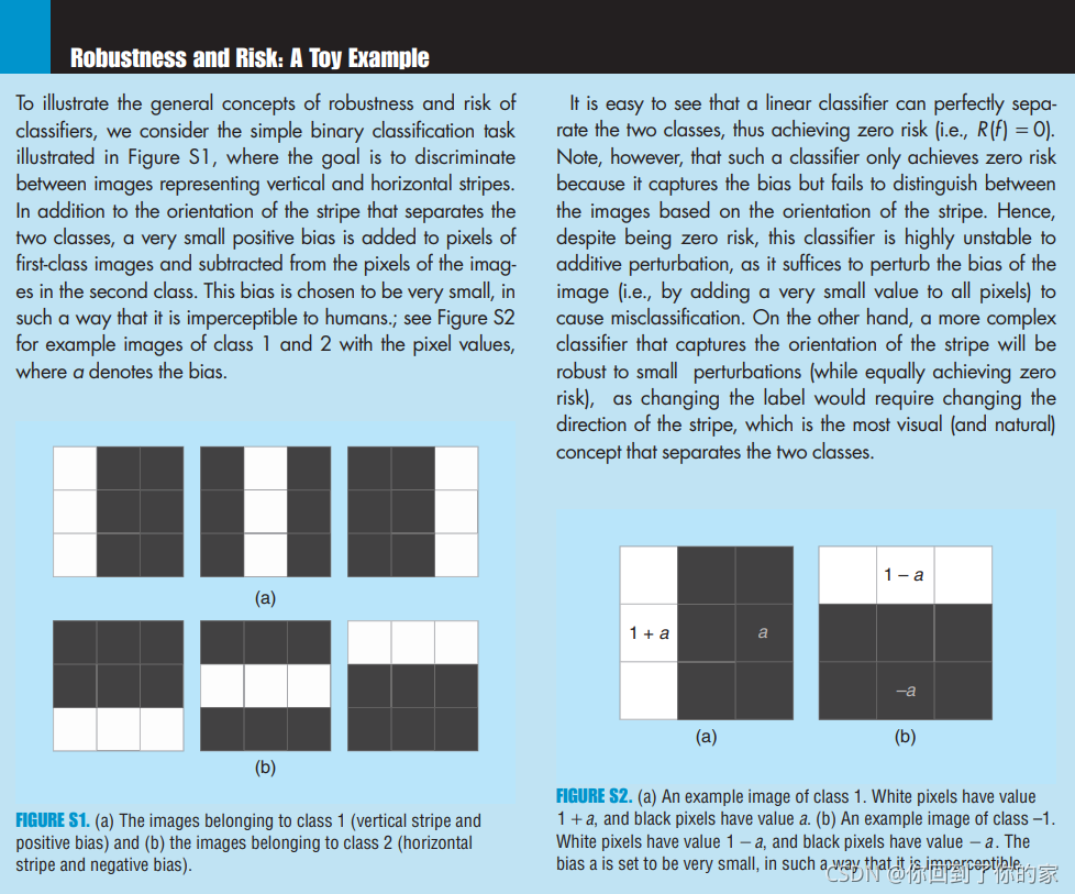
Observe that classification robustnessºÍÖ§³ÖÏòÁ¿»úclassifierÓнÏÇ¿µÄ¹ØÁª，ºóÕßµÄÄ¿±êÊÇ×î´ó»¯robustness，defined as the margin between support vectors. Importantly, the max-margin classifier in a given family of classifiers might, however, still not achieve robustness (in the sense of high $¦Ñ(f)$). An illustration is provided in ¡°Robustness and Risk: A Toy Example,¡± where a no zero-risk linear classifier¡ªin particular, the max-margin classifier¡ª achieves robustness to perturbations. Our focus in this article is turned toward assessing the robustness of the family of deep neural network classifiers that are used in many visual recognition tasks.

Perturbation forms

Robustness to additive perturbations

We first start by considering the case where the perturbation operator is simply additive，¼´$T_r(x)=x+r$¡£ÔÚÕâÖÖÇé¿öÏÂ, the magnitude of the perturbation can be measured with the $l_p$ norm of the minimal perturbation that is necessary to change the label of a classifier. According to (2), the robustness to additive perturbations of a data point x is defined as：

$$\begin{gathered} \underset{r¡Ê\mathcal{R}}{\min }¡Îr{¡Î}_p \\ subjecttof(x+r)ªÁ=f(x)(4) \end{gathered}$$

Depending on the conditions that one sets on the set $\mathcal{R}$ that supports the perturbations, the additive model leads to different forms of robustness.

Adversarial perturbations

ÎÒÃÇÊ×ÏÈ¿¼ÂÇadditive perturbations²»ÊÜÏÞÖƵÄÇé¿ö，¼´$\mathcal{R}=\mathcal{X}$¡£Í¨¹ý½â¾ö（4）µÃµ½µÄperturbationͨ³£±»³Æ×÷adversarial perturbation, as it corresponds to the perturbation that an adversary (having full knowledge of the model) would apply to change the label of the classifier, while causing minimal changes to the original image.

The optimization problem in (4) is nonconvex, as the constraint involves the (potentially highly complex) classification function $f$. Different techniques exist to approximate adversarial perturbations. In the following, we briefly mention some of the existing algorithms for computing adversarial perturbations:

Regularized variant[1]： ÕâÖÖ·½Ê½Í¨¹ý½â¾öa regularized variant of the problem in （4）À´»ñÈ¡adversarial perturbation，Õâ¸ö±äÖÖÎÊÌâ¿ÉÒÔÓÃÈçÏµĹ«Ê½½øÐÐÃèÊö：

$$\underset{r}{\min }c¡Îr{¡Î}_p+J(x+r,\tilde{y},¦È)(5)$$

ÕâÀï$\tilde{y}$ÊÇperturbed sampleµÄtarget label，$J$ÊÇloss function，$c$ÊÇÒ»¸öregularization ²ÎÊý，$¦È$ÊÇÄ£ÐͲÎÊý¡£ÔÚ[1]ÖÐ×îԭʼµÄ¹«Ê½ÖÐ，Ìí¼ÓÁËÒ»¸ö¶îÍâµÄ±äÁ¿ÏÞÖÆÀ´±£Ö¤$x+r¡Ê[0,1]$，ÕâÔÚ（5）ÖÐΪÁ˼òµ¥ÐÔ½øÐÐÁËÊ¡ÂÔ¡£ÎªÁ˽â¾ö（5）ÖеÄÓÅ»¯ÎÊÌâ，a line search is performed over $c$ to find the maximum $c>0$ for which the minimizer of (5) satisfies $f(x+r)=\tilde{y}$¡£¾¡¹Ü¿ÉÒÔ²úÉú·Ç³£¾«×¼µÄ¹À¼Æ，ÕâÖÖ·½·¨can be costly to compute on high-dimensional and large-scale datasets¡£Moreover，it computes targeted adversarial perturbation，where the target label is known¡£

Fast gradient sign(FGS)[11]：ÕâÖÖ·½Ê½Í¨¹ýgoing in the direction of the sign of gradient of the loss functionÀ´¹À¼Æan untargeted adversarial perturbation，loss function¶¨ÒåÈçÏÂ：

$$?sign({?}_{x}J(x,y(x),¦È))$$

ÕâÀï$J$ÊÇloss function，ÓÃÀ´ÑµÁ·Éñ¾­ÍøÂç²¢ÇÒ$¦È$±íʾģÐͲÎÊý¡£¾¡¹ÜÊ®·Ö¸ßЧ，ÕâÖÖone-stepµÄËã·¨½öÄÜÌṩa coarse approximation to the solution of the optimization problem in （4） for $p=¡Þ$

DeepFool[5]： Õâ¸öË㷨ͨ¹ýÒ»¸öµü´úµÄ²½ÖèÀ´×îС»¯（4），where each iteration involves the linearization of the constraint¡£The linearized （constrained）problem is solved in closed form at each iteration，and the current estimate is updated；ÓÅ»¯¹ý³Ìµ±µ±Ç°µÄestimate of the perturbation fools the classifierʱÖÕÖ¹¡£In practice，DeepFool provides a tradeoff between the accuracy and efficiency of the two previous approaches¡£

In addition to the aforementioned optimization methods, several other approaches have recently been proposed to compute adversarial perturbations, see, e.g., [9], [12], and [13]. Different from the previously mentioned gradient-based techniques, the recent work in [14] learns a network (the adversarial transformation network) to efficiently generate a set of perturbations with a large diversity, without requiring the computation of the gradients.

ʹÓÃÏÈÇ°Ìá¼°µ½µÄÕâЩ¼¼ÇÉ， one can compute the robustness of classifiers to additive adversarial perturbations. Quite surprisingly, deep networks are extremely vulnerable to such additive perturbations; i.e.,
small and even imperceptible adversarial perturbations can be computed to fool them with high probability. For example, the average perturbations required to fool the CaffeNet [15] and GoogleNet [16] architectures on the ILSVRC 2012 task [17] are 100 times smaller than the typical norm of natural images [5] when using the $l_2$ norm. The high instability of deep neural networks to adversarial perturbations, which was first highlighted in [1], shows that these networks rely heavily on proxy concepts to classify objects, as opposed to strong visual concepts typically used by humans to distinguish between objects.

To illustrate this idea, we consider once again the toy classification example (see ¡°Robustness and Risk: A Toy Example¡±), where the goal is to classify images based on the orientation of the stripe. In this example, linear classifiers could achieve a perfect recognition rate by exploiting the imperceptibly small bias that separates the two classes. While this proxy concept achieves zero risk, it is not robust to perturbations: one could design an additive perturbation that is as simple as a minor variation of the bias, which is sufficient to induce data misclassification. On the same line of thought, the high instability of classifiers to additive perturbations observed in [1] suggests that deep neural networks potentially capture one of the proxy concepts that separate the different classes. Through a quantitative analysis of polynomial classifiers, [10] suggests that higher-degree classifiers tend to be more robust to perturbations, as they capture the ¡°stronger¡± (and more visual) concept that separates the classes (e.g., the orientation of the stripe in Figure S1 in ¡°Robustness and Risk: A Toy Example¡±). For neural networks, however, the relation between the flexibility of the architecture (e.g., depth and breadth) and adversarial robustness is not well understood and remains an open problem.

Random noise

´ý²¹³ä

Geometric insights from robustness

¶ÔrobustnessµÄÑо¿ÔÊÐíÎÒÃÇ»ñµÃ¹ØÓÚclassifierµÄinsights，¸ü׼ȷµØ½²，ÊǹØÓÚthe geometry of the
classification function acting on the high-dimensional input space. f : X ¡ú { 1 , ] ¡­ , C } f:\mathcal{X}\to\{1,]\dots,C\} f:X¡ú{1,]¡­,C}Ö¸´úÎÒÃǵÄC-class·ÖÀàÆ÷, ²¢ÇÒÎÒÃÇÓÃ$g_1,¡­,g_c$ ±íʾ·ÖÀàÆ÷¶Ô$C$¸öÀàÖеÄÿ¸öÅж¨µÄ¸ÅÂÊ¡£ÌرðµØ，¶ÔÓÚÒ»¸ö¸ø¶¨µÄ$x¡Ê\mathcal{X}$, $f(x)$ is assigned to the class having a maximal score，¼´ f ( x ) = a r g m a x i { ( g i ( x ) } f(x)=argmax_i\{(g_i(x)\} f(x)=argmaxi?{(gi?(x)}¡£¶ÔÓÚÉî¶ÈÉñ¾­ÍøÂç，º¯Êý$g_i$´ú±íÍøÂçÖÐ×îºóÒ»²ãµÄÊä³ö（ͨ³£Ö¸softmax²ã）¡£Note that the classifier $f$ can be seen as a mapping that partitions the input space $\mathcal{X}$ into classification regions, each of which has a constant estimated label (i.e., $f(x)$ is constant for each such region). The decision boundary $\mathcal{B}$ of the classifier is defined as the union of the boundaries of such classification regions (see Figure 2).

Adversarial perturbations

ÎÒÃÇÊ×ÏȾ۽¹ÓÚadversarial perturbation²¢ÇÒhighlightÕâЩÈŶ¯ºÍ¾ö²ß±ß½ç¼¸ºÎ½á¹¹µÄ¹Øϵ¡£ÕâÖÖ¹Øϵrelies on the simple observation shown in ¡°Geometric Properties of Adversarial Perturbations.¡±¡£Á½¸ö¼¸ºÎÐÔÖʶ¼ÔÚͼ6ÖнøÐÐÁËչʾ：

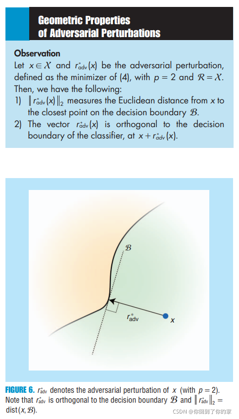
×¢ÒâÕâЩ¼¸ºÎÐÔÖÊare specific to the $l_2$·¶Êý The high instability of classifiers to adversarial perturbations, which we highlighted in the previous section, ½ÒʾÁË×ÔȻͼƬ¶¼Î»Óڷdz£½Ó½üÓÚ¾ö²ß±ß½çµÄλÖ᣾¡¹ÜÕâ¸ö½á¹ûÊÇÀí½âthe geometry of the data points with regard to the classifier¡®s¾ö²ß±ß½çµÄ¹Ø¼ü，Ëü²¢Ã»ÓÐÌṩÈκÎÓйØÓÚ¾ö²ß±ß½çÐÎ×´µÄinsight . Ò»¸ö¹ØÓÚ¾ö²ß±ß½çµÄlocal geometricÃèÊö (λÓÚ$x$µÄÖÜΧµØÇø) is rather capturedͨ¹ý$r_{adv}^{?}(x)$µÄ·½Ïò，due to adversarial perturbationµÄ´¹Ö±ÐÔ. In [18] and [25], ÕâЩadversarial perturbationµÄ¼¸ºÎÐÔÖʱ»ÀûÓÃÀ´½øÐÐÔÚÊý¾ÝµãµÄÖÜΧµØÇø¿ÉÊÓ»¯¾ö²ß±ß½çµÄtypical cross sections. ÌرðµØ，a two-dimensional normal section of the decision boundary is illustrated, where the sectioning plane is spanned by the adversarial perturbation (´¹Ö±ÓÚ¾ö²ß±ß½ç) and a random vector in the tangent space. Examples of normal sections of decision boundaries are illustrated in Figure 7：

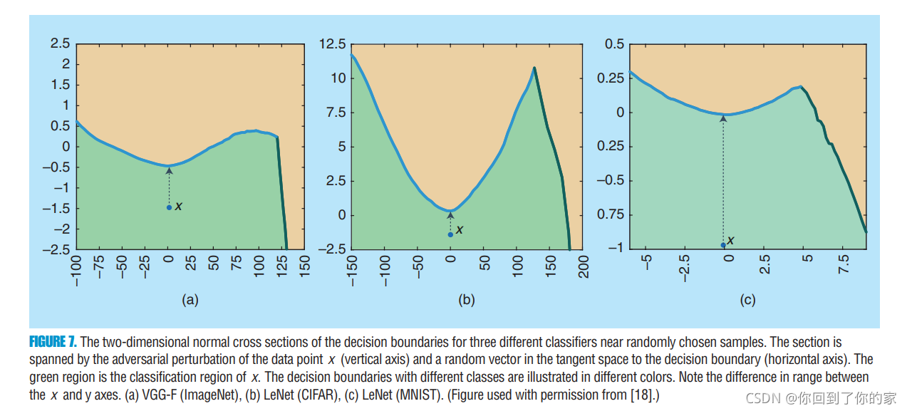
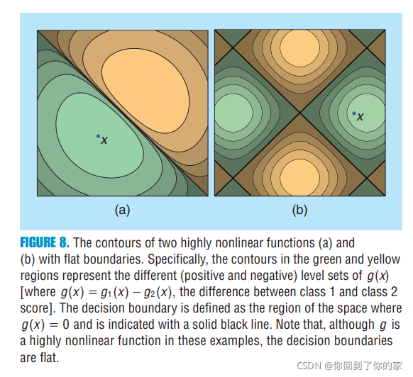
ÎÒÃÇ¿ÉÒԹ۲쵽SOTAÉî¶ÈÉñ¾­ÍøÂçµÄ¾ö²ß±ß½çon these two-dimensional cross sectionsÓÐÒ»¸ö·Ç³£µÍµÄcurvature (×¢ÒâxÖáºÍyÖáµÄÇø±ðn)¡£»»¾ä»°Ëµ，ÕâЩͼ±í½ÒʾÁË$x$¸½½üλÖõľö²ß±ß½çcan be locally well approximated by a hyperplane passing through $x+r_{adv}^{?}(x)$ with the normal vector $r_{adv}^{?}(x)$¡£ In [11], it is hypothesized that state-of-the-art classifiers are ¡°too linear,¡± µ¼ÖÂÁ˾ö²ß±ß½çwith very small curvature²¢½øÒ»²½½âÊÍÁË the high instability of such classifiers to adversarial perturbations. To motivate the linearity hypothesis of deep networks, the success of the FGS method (which is exact for linear classifiers) in finding adversarial perturbations is invoked. È»¶ø，×î½üµÄһЩ¹¤×÷¶ÔÏßÐÔ¼ÙÉè×ö³öÁËÌôÕ½，ÀýÈç[26], the authors show that there exist adversarial perturbations that cannot be explained with this hypothesis, and, in [27], the authors provide a new explanation based on the tilting of the decision boundary with respect to the data manifold. We stress here that the low curvature of the decision boundary does not, in general, imply that the function learned
by the deep neural network (as a function of the input image) is linear, or even approximately linear. Figure 8 shows illustrative examples of highly nonlinear functions resulting in flat decision boundaries.：

Moreover, it should be noted that, while the decision boundary of deep networks is very flat on random two-dimensional cross sections, these boundaries are not flat on all cross sections. That is, there exist directions in which the boundary is very curved. Figure 9 provides some illustrations of such cross sections, where the decision boundary has large curvature and therefore significantly departs from the first-order linear approximation, suggested by the flatness of the decision boundary on random sections in Figure 7.：

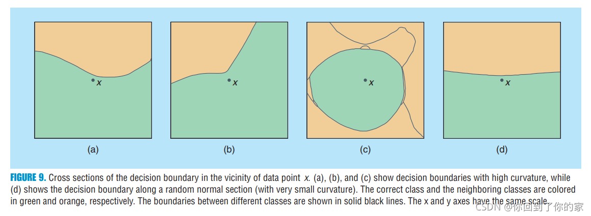
Hence, these visualizations of the decision boundary strongly suggest that the curvature along a small set of directions can be very large and that the curvature is relatively small along random directions in the input space. Using a numerical computation of the curvature, the sparsity of the curvature profile is empirically verified in [28] for deep neural networks, and the directions where the decision boundary is curved are further shown to play a major role in explaining the robustness properties of classifiers. In [29], the authors provide a complementary analysis on the curvature of the decision boundaries induced by deep networks and show that the first principal curvatures increase exponentially with the depth of a random neural network. The analyses of [28] and [29] hence suggest that the curvature profile of deep networks is highly sparse (i.e., the decision boundaries are almost flat along most directions) but can have a very large curvature along a few directions.

Universal perturbations

´ý²¹³ä