[人工智能] Machine Learning - Coursera 吴恩达机器学习教程 Week1 学习笔记

开发: C++知识库 Java知识库 JavaScript Python PHP知识库人工智能区块链大数据移动开发嵌入式开发工具数据结构与算法开发测试游戏开发网络协议系统运维
教程: HTML教程 CSS教程 JavaScript教程 Go语言教程 JQuery教程 VUE教程 VUE3教程 Bootstrap教程 SQL数据库教程 C语言教程 C++教程 Java教程 Python教程 Python3教程 C#教程
数码: 电脑笔记本显卡显示器固态硬盘硬盘耳机手机 iphone vivo oppo 小米华为单反装机图拉丁

-> 人工智能 -> Machine Learning - Coursera 吴恩达机器学习教程 Week1 学习笔记 -> 正文阅读

[人工智能]Machine Learning - Coursera 吴恩达机器学习教程 Week1 学习笔记

机器学习的定义

Arthur Samuel 传统定义

Arthur Samuel: “the field of study that gives computers the ability to learn without being explicitly programmed.” This is an older, informal definition.

让计算机无需明确编程，就有学习能力。

Tom Mitchell 现代定义

Tom Mitchell: “A computer program is said to learn from experience E with respect to some class of tasks T and performance measure P, if its performance at tasks in T, as measured by P, improves with experience E.”

若一个程序能从某任务T的经验E中学习后，提高任务T的性能P，就可以成之为机器学习。

比如下棋的例子：

E：下许多盘棋的经验
T：下棋
P：下一盘棋的胜率

通常，机器学习算法可分为两大类：有监督学习和无监督学习。

有监督学习（Supervised Learning）

有监督学习：提供了正确答案。

主要分为回归和分类。

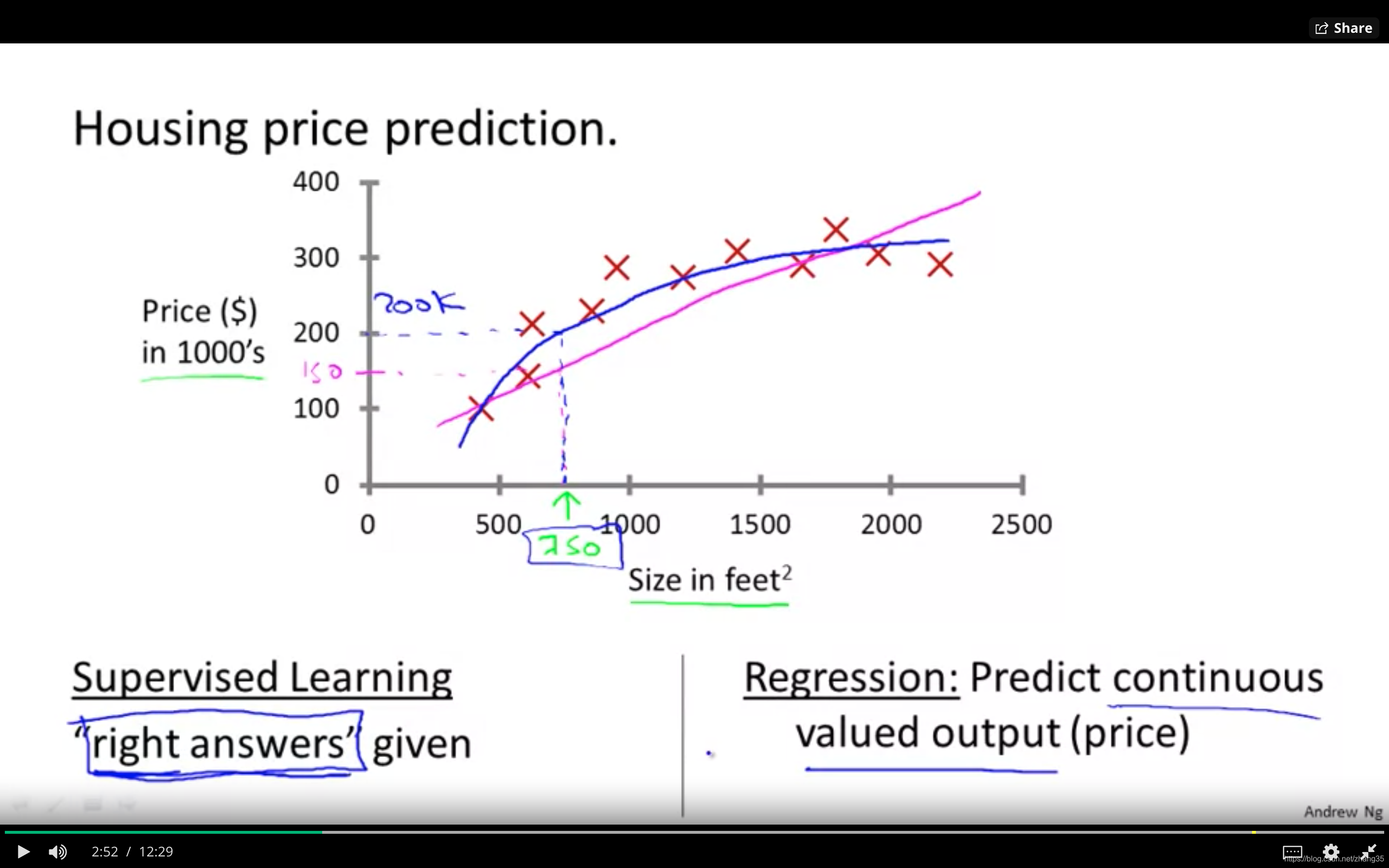
回归（Regression）

需预测的目标变量连续时，比如房价和面积的关系，为线性回归问题；
在这里插入图片描述

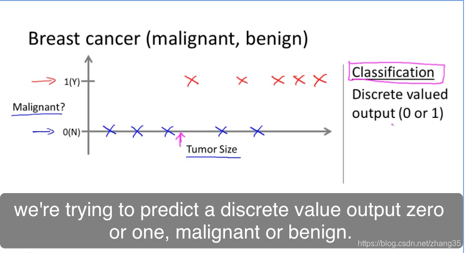
分类（Classification）

只有离散的几种取值时，比如肿瘤是否是良性，则为分类问题。
在这里插入图片描述
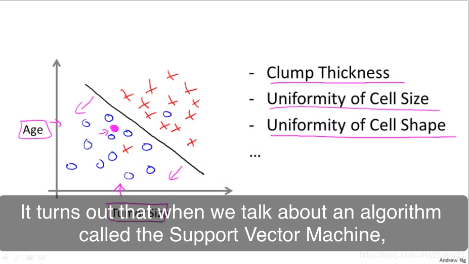
需要分类的属性太多，就需要用到支持向量机：

无监督学习（Unsupervised Learning）

无监督学习：不提供参考答案。只能从数据本身的关联中提取模式。

聚类: 给你1,000,000个不同的基因，通过不同的变量如寿命、位置、角色等，将它们自动分类。

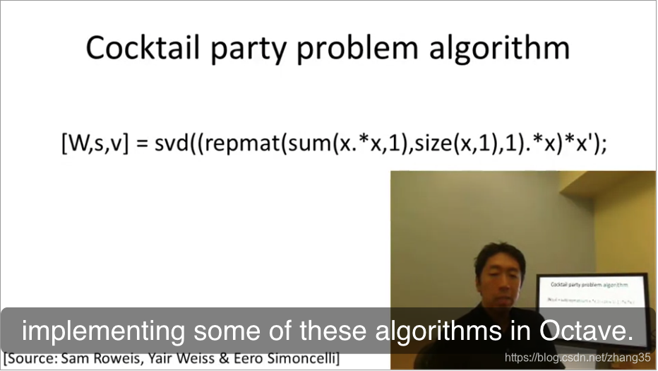
非聚类：鸡尾酒聚会算法，能在嘈杂环境中识别出背景音乐和不同个体的声音。
![在这里插入图片描述](https://img-blog.csdnimg.cn/20
鸡尾酒聚会问题，一行代码解决：

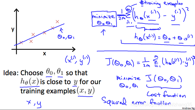
模型

在这里插入图片描述
x⁽ⁱ⁾ ：输入变量
y⁽ⁱ⁾ ：目标变量
h(x) ：hypothesis，假设的目标函数

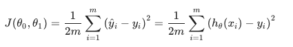
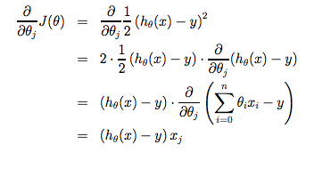
代价函数

J(θ) 代表目标函数和原始函数见的差距，即代价函数。

使得J(θ)最小的那个h(x)就是预期的目标函数。

最常用的J(θ)表示如下，也叫做均方差函数：
在这里插入图片描述

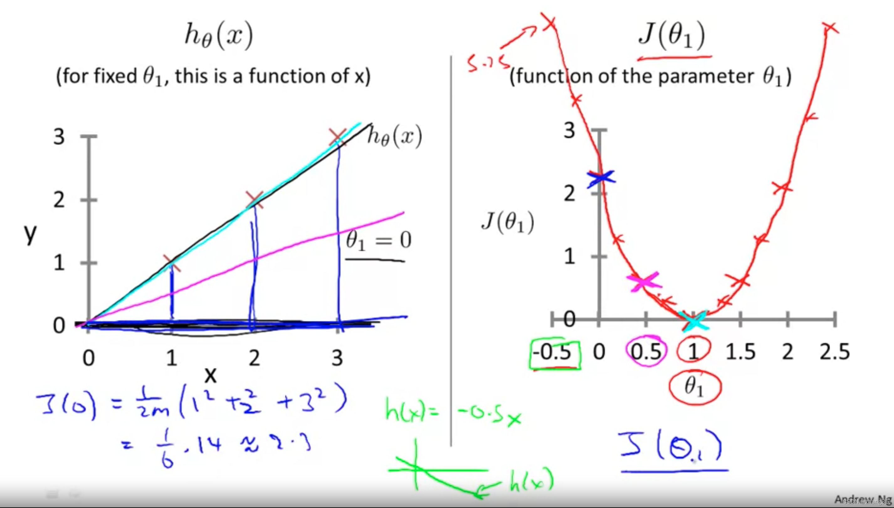
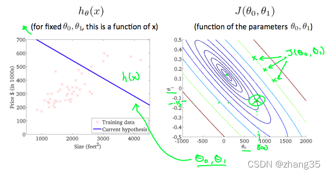
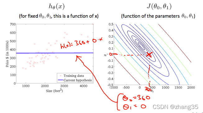
当J(θ₀)只有一个变量时，J随θ的变化是二维图像：
在这里插入图片描述

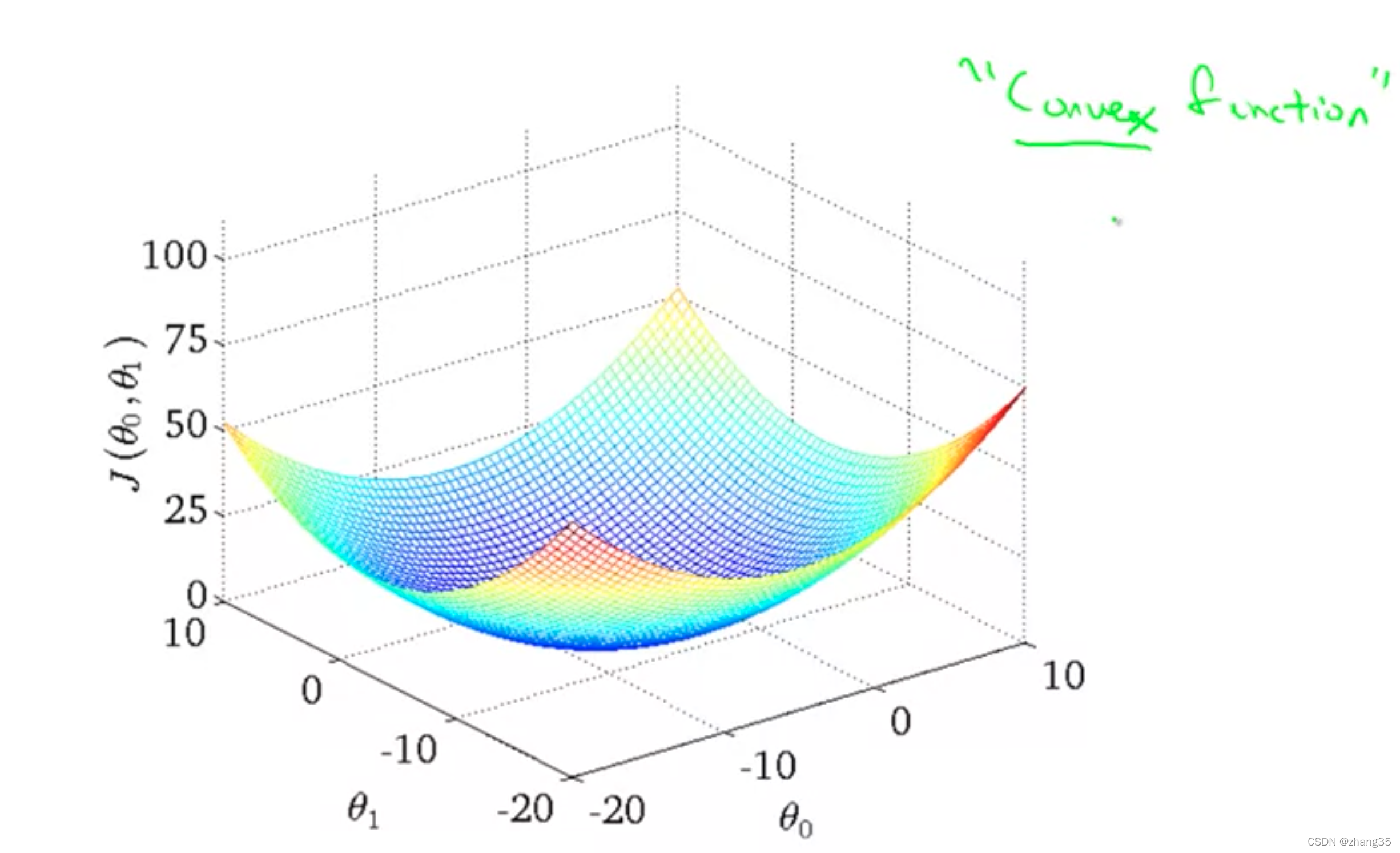
当J(θ₀, θ₁)有两个变量时，函数图是三维的：
在这里插入图片描述
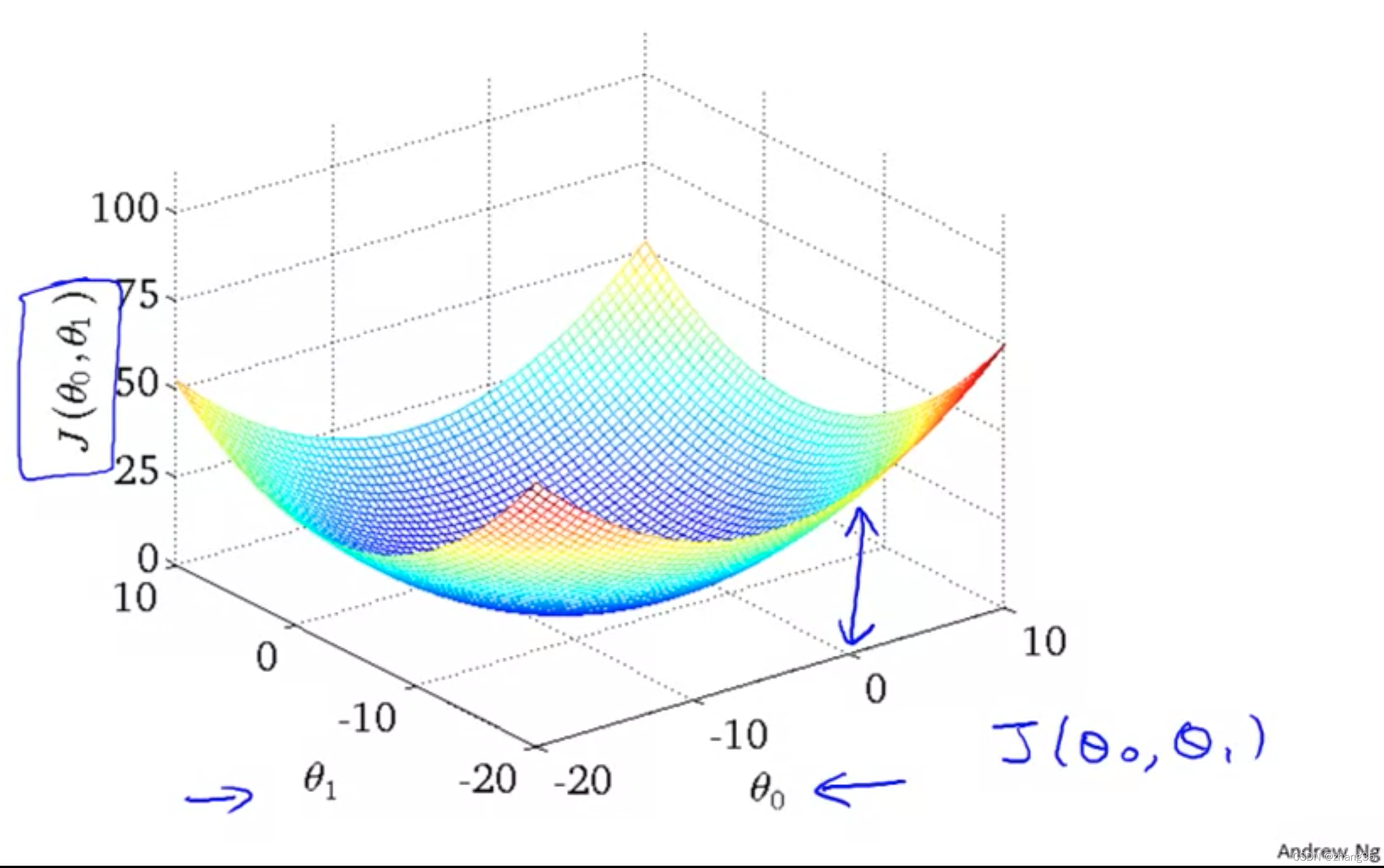
可以用等高线来表示取得相同J值的θ₀和θ₁。

右图从等高线外围到中心，J的值越来越小，可以看到对应左侧的h(x)越来越靠谱：
在这里插入图片描述

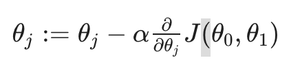
梯度下降（gradient descent）

寻找最佳目标函数h(x)的过程，也即最小化代价函数J(θ)的过程。

目标就是找到让J(θ)最小的θ值。

寻找最小θ值，一般用梯度下降法。

这里需要认识一些术语：

derivative term 导数项
Partial Derivative 偏导数
multivariate 多元
convergent 收敛
calculus 微积分
tangent 切线；正切
convex function 凸函数（碗状的）
Quadratic function：二次函数

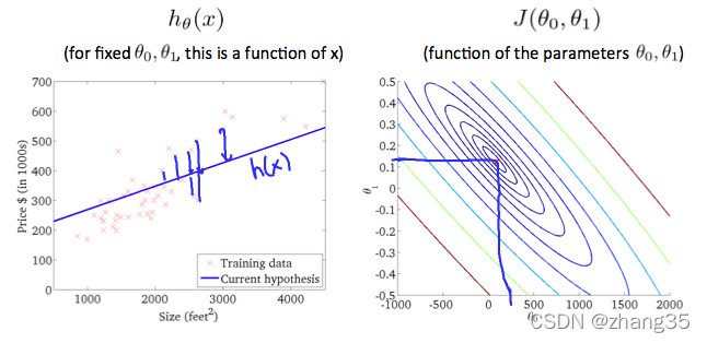
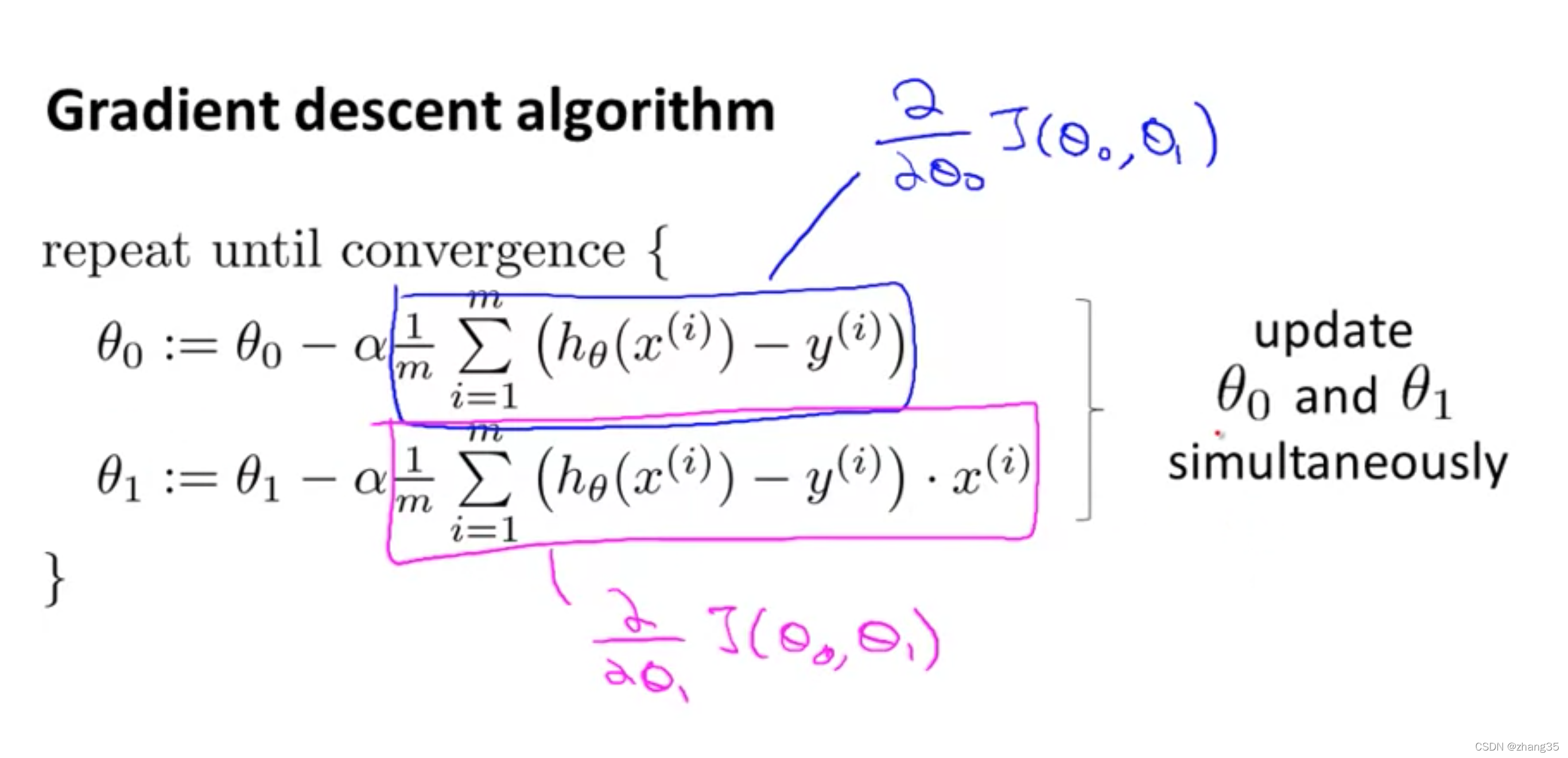
梯度下降法公式：重复以下式子，直到收敛。
在这里插入图片描述

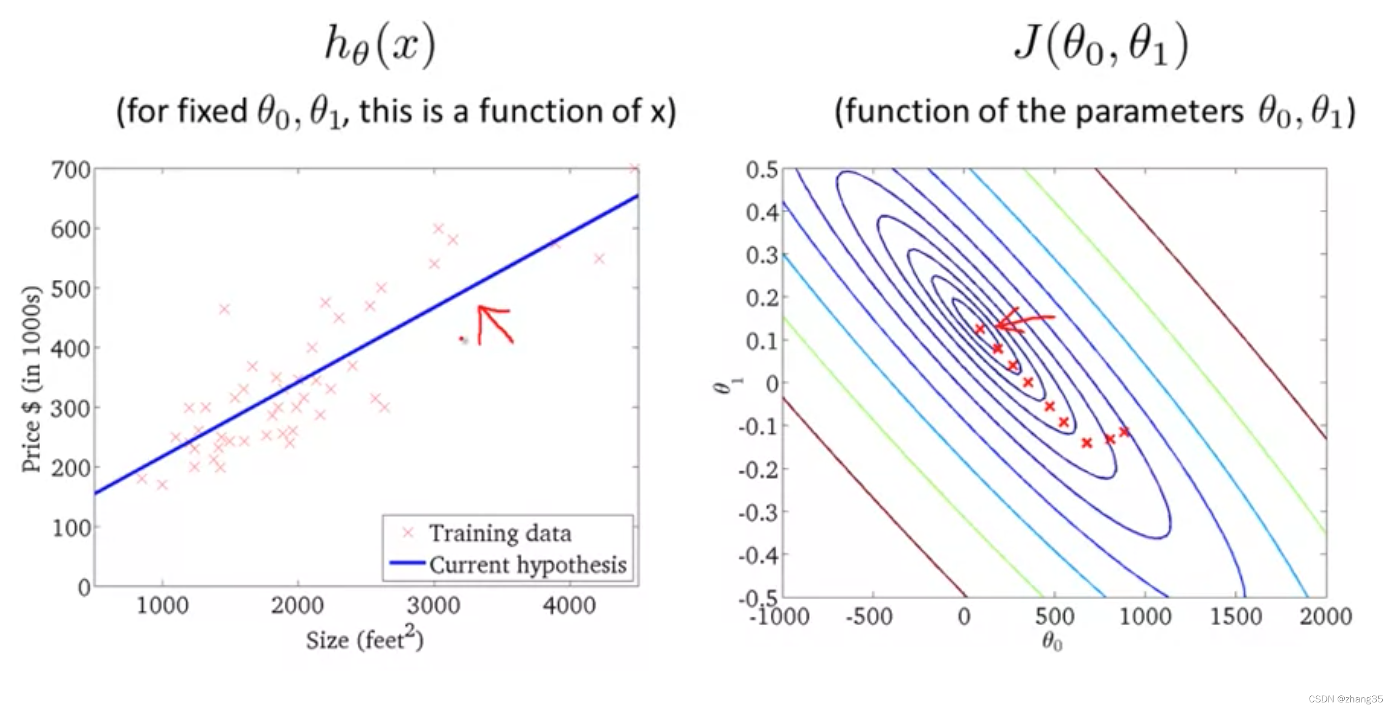
求解过程如下图，每个星星是一步。

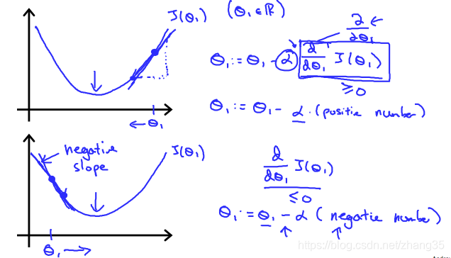
α：学习率，α越大，步子越大；

J的偏导数，从几何意义上讲，就是函数变化增加最快的地方。朝着下降最多的方向进行；

不同的起点，会带来不同的下降方向，如下图：
在这里插入图片描述
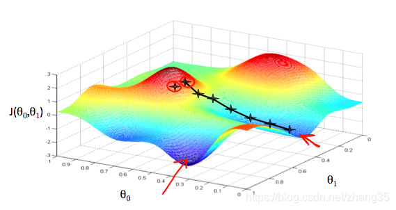
θ₀, θ₁的起始值其实无关紧要，一般均初始化为0。

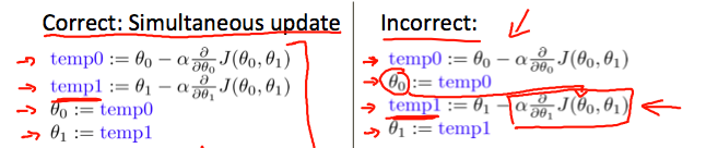
梯度下降，一定要同步更新多个变量，否则就会出错：
在这里插入图片描述

朝着梯度下降的方向逐渐收敛，在斜率为正的地方会减小，斜率为负的地方会增大，就是为了滑到谷底。
在这里插入图片描述
a过小时，收敛速度会过慢；

a过大时，步子迈得太大，甚至可能会发散。
在这里插入图片描述
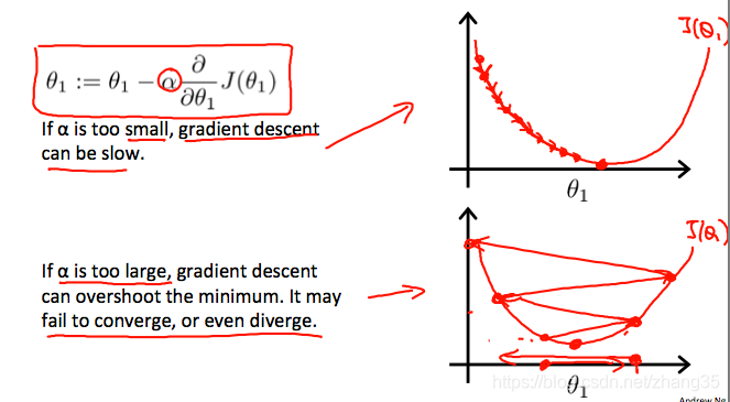
固定的a也能自动减小step，因为导数在逐渐减小：
所以不用手动减小a。

例子：线性回归中的梯度下降

线性回归中，J是一个凸函数，所以总是能到达全局最优解：
在这里插入图片描述
偏导数如下：

此时梯度下降公式就变成了：

每步梯度下降，对应的图像化表示为：

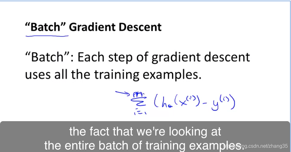
线性回归使用了批量梯度下降：即每步都使用所有的训练集。

其它梯度下降算法可能仅使用一个子集的训练数据。
在这里插入图片描述

至此学习了第一个机器学习算法，基于梯度下降法的线性回归问题——机器学习界的Hello World。

线性代数复习

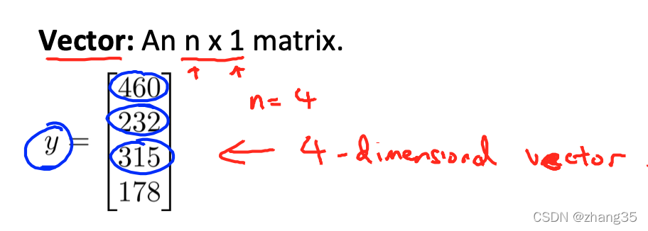
Vector ： n * 1矩阵
R⁴ : 4维向量

在这里插入图片描述
没有特殊说明时，该课程的下标i从1计数。

一些术语：
单位矩阵：identity matrix
singular matrix：奇异矩阵
degenerate matrix：退化矩阵

常用的Octave/Matlab代码

矩阵和向量

向量：一个n * 1的矩阵，相当于一列
在这里插入图片描述

% The ; denotes we are going back to a new row.
A = [1, 2, 3; 4, 5, 6; 7, 8, 9; 10, 11, 12]

% Initialize a vector 
v = [1;2;3] 

% Get the dimension of the matrix A where m = rows and n = columns
[m,n] = size(A)

% You could also store it this way
dim_A = size(A)

% Get the dimension of the vector v 
dim_v = size(v)

% Now let's index into the 2nd row 3rd column of matrix A
A_23 = A(2,3)

输出：

A =

    1    2    3
    4    5    6
    7    8    9
   10   11   12

v =

   1
   2
   3

m =  4
n =  3
dim_A =

   4   3

dim_v =

   3   1

A_23 =  6

加法和标量乘法

% Initialize matrix A and B 
A = [1, 2, 4; 5, 3, 2]
B = [1, 3, 4; 1, 1, 1]

% Initialize constant s 
s = 2

% See how element-wise addition works
add_AB = A + B 

% See how element-wise subtraction works
sub_AB = A - B

% See how scalar multiplication works
mult_As = A * s

% Divide A by s
div_As = A / s

% What happens if we have a Matrix + scalar?
add_As = A + s

输出：

A =

   1   2   4
   5   3   2

B =

   1   3   4
   1   1   1

s =  2
add_AB =

   2   5   8
   6   4   3

sub_AB =

   0  -1   0
   4   2   1

mult_As =

    2    4    8
   10    6    4

div_As =

   0.50000   1.00000   2.00000
   2.50000   1.50000   1.00000

add_As =

   3   4   6
   7   5   4

矩阵乘以向量

% Initialize matrix A 
A = [1, 2, 3; 4, 5, 6;7, 8, 9] 

% Initialize vector v 
v = [1; 1; 1] 

% Multiply A * v
Av = A * v

输出：

矩阵乘以矩阵

% Initialize a 3 by 2 matrix 
A = [1, 2; 3, 4;5, 6]

% Initialize a 2 by 1 matrix 
B = [1; 2] 

% We expect a resulting matrix of (3 by 2)*(2 by 1) = (3 by 1) 
mult_AB = A*B

% Make sure you understand why we got that result

输出：

乘法性质

不满足交换律：A?B != B?A
满足结合律：(A?B)?C = A?(B?C)
单位矩阵（ identity matrix）：A * I = I * A = A

% Initialize random matrices A and B 
A = [1,2;4,5]
B = [1,1;0,2]

% Initialize a 2 by 2 identity matrix
I = eye(2)

% The above notation is the same as I = [1,0;0,1]

% What happens when we multiply I*A ? 
IA = I*A 

% How about A*I ? 
AI = A*I 

% Compute A*B 
AB = A*B 

% Is it equal to B*A? 
BA = B*A 

% Note that IA = AI but AB != BA

输出：

A =

   1   2
   4   5

B =

   1   1
   0   2

I =

Diagonal Matrix

   1   0
   0   1

IA =

   1   2
   4   5

AI =

   1   2
   4   5

AB =

    1    5
    4   14

BA =

    5    7
    8   10

逆矩阵和转置矩阵

矩阵和逆矩阵相乘，得到单位矩阵：

A * A^-1 = I

转置矩阵是顺时针旋转90°，然后在水平翻转一下。

% Initialize matrix A 
A = [1,2,0;0,5,6;7,0,9]

% Transpose A 
A_trans = A' 

% Take the inverse of A 
A_inv = inv(A)

% What is A^(-1)*A? 
A_invA = inv(A)*A

输出：

A =

   1   2   0
   0   5   6
   7   0   9

A_trans =

   1   0   7
   2   5   0
   0   6   9

A_inv =

   0.348837  -0.139535   0.093023
   0.325581   0.069767  -0.046512
  -0.271318   0.108527   0.038760

A_invA =

   1.00000  -0.00000   0.00000
   0.00000   1.00000  -0.00000
  -0.00000   0.00000   1.00000