Pytorch实现机器学习之线性回归2.0

一、Pytorch实现机器学习之线性回归1.0，特点在利用tensor手动实现线性回归反向传播。

点击打开《Pytorch实现机器学习之线性回归》文章

二、Pytorch实现机器学习之线性回归2.0，特点在利用autograd和Variable实现线性回归，并且反向传播自动调用backward实现。

import torch as t
from matplotlib import pyplot as plt
from IPython import display
from torch.autograd import Variable as V
t.manual_seed(10) # 设置随机数种子

def get_randn_data(batch_size=8):
    """产生随机数x并给线性函数y=2x+3加上噪声，便于后面学习能否贴近结果"""
    x = t.randn(batch_size,1)*20
    y = x * 2 + (1 + t.randn(batch_size,1))*3
    return x,y

# 随机初始化参数w和零初始化参数b，variable格式
w = V(t.randn(1,1),requires_grad=True)
b = V(t.zeros(1,1),requires_grad=True)

# 设置学习率或者步长
lr = 0.0001

# 创建列表分别存储参数w和b的变化值
listw = []
listb = []

for count in range(20000): # 训练20000次并测试输出
    # 训练过程
    x,y = get_randn_data() # x,y都是真实数据也就是实际值
    x,y = V(x),V(y) # tensor转换成variable

    # 前向传播，从头往后传到得出预测值，再得出损失函数下损失值
    y_p = x.mm(w) + b.expand_as(y) # 实现的就是通过参数w和b和因变量x计算预测值y_p = wx + b
    loss = 0.5 * (y_p - y) ** 2 # 实现的就是计算损失函数的损失值loss = 1/2(y_p - y) ** 2
    loss = loss.sum() # loss为variable格式，所以要计算损失函数的值需要全部加起来得出总和

    # 反向传播,自行计算梯度
    # loss.backward(t.ones(loss.size())) # 当loss非一维variable时采用
    loss.backward()

    # 相减实现梯度下降,更新参数w和b,因为variable本身不能实现inplace操作，所以要将w和b从variable转换成tensor，data存储是tensor
    w.data.sub_(lr * w.grad.data)
    b.data.sub_(lr * b.grad.data)

    # 梯度清零
    w.grad.data.zero_()
    b.grad.data.zero_()

    # 测试输出过程
    # 每训练1000次输出训练实现预测结果一次,画图（线和散点）
    if count % 1000 == 0:

        # 设置画图中横纵坐标的范围
        plt.xlim(0,20)
        plt.ylim(0,45)

        display.clear_output(wait=True) # 清空并显示实时数据动态表示
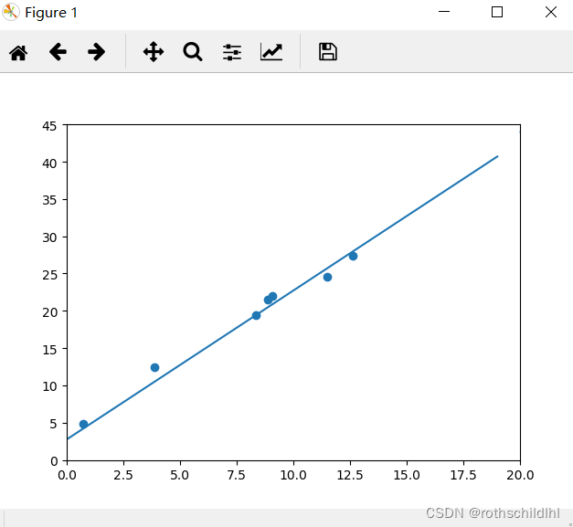
        # 训练得到的函数模型显示的线性图形
        x1 = t.arange(0,20).view(-1,1) # view为-1时会tensor根据元素自动计算维度大小
        x1 = x1.float()
        y1 = x1.mm(w.data) + b.data.expand_as(x1) # 计算需要的是tensor格式而非variable
        plt.plot(x1.squeeze().numpy(),y1.squeeze().numpy())

        # 随机生成的测试数据，用来检验函数模型是否匹配随机测试数据点状图形
        x2,y2 = get_randn_data(batch_size=20)
        plt.scatter(x2.squeeze().numpy(),y2.squeeze().numpy())

        # 图像输出并在2秒后自动关闭
        plt.show(block=False)
        plt.pause(2)
        plt.close()

        # 输出每次训练后的模型参数w和b的值，也可以看出w和b的变化趋势
        # print(w.squeeze().numpy(), b.squeeze().numpy())

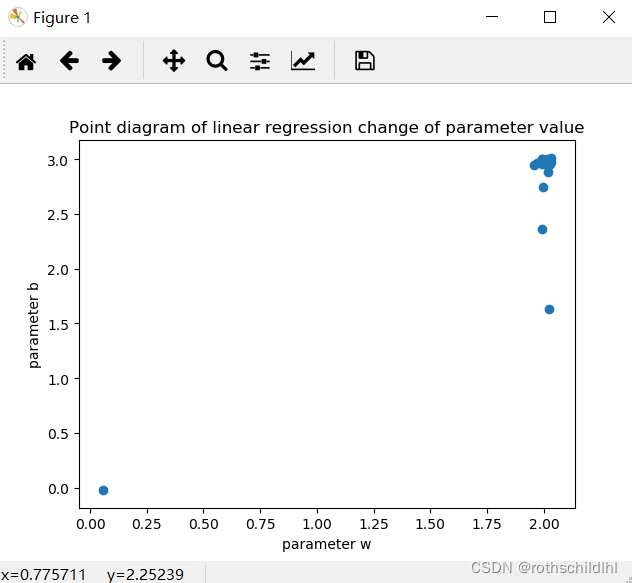
        # 收集参数w和b每次训练变化的值，实现后面参数值线性回归变化点状图的显示
        listw.append((w.data.squeeze().numpy().tolist())) # tensor->numpy->list
        listb.append((b.data.squeeze().numpy().tolist()))

# 参数值线性回归变化点状图的显示
plt.title("Point diagram of linear regression change of parameter value")
plt.xlabel("parameter w")
plt.ylabel("parameter b")
plt.scatter(listw,listb)
plt.show(block=False)
plt.pause(10)
plt.close()