Applied Machine Learning

Introduction

Terms

A dataset that is intended to be analyzed by machine learning method is supposed to have Feature (X) and Target Value/Label (y)

Traning and test sets are needed for a given dataset.
Model fitting will produce a ‘training model’ by using the training set of data. Then, we can evaluate the model based on the training model.

There are two types of problems in machine learning: classfication and regression. Both catrgories take a set of traning instances and learn a mapping to produce a target value. Classification return discret value, while Regression return continuous value.

Overfitting and Underfitting

Generalization ability refers to an algorithm’s ability to give accurate predictions for new previously unseen data.

Overfit Models are too complex. Not likely to generalize well to new examples.
Underfit Models are too simple. Not do well on training data.

Supervised Learning

k-Nearest Neighbor

Find the most similar (closest) instances (in X_train) to the x_test
Get the corresponding y_label of the X_train
Predict the label for x_test by combing label acquired from the 2nd step.

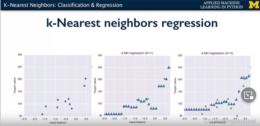
Beyond classification, knn can be used for regression. Simply find the closest output value corresponding to the features. 在这里插入图片描述

Linear Model

It is a sum of weighted variables that predicts a target output calue given an input data instance.
(eg: predicting housing prices, (ax + by + cz = target_value)

Input feature vector: x = (x0, x1, x2…)
Parameters to estimate
w = (w0,w1,w2…) slope
b = (b0,b1,b2…) constant bias

Least Squares

Finds the w and b that minimizes the mean squared error of the model: the sum of squared differences between predicted target and actual target values.

No parameters to control model complexity.

Parameters (w,b) are estimated from training data. The learning algorithm would want to minimize a loss function.

Loss function in this case is Sum of squared differences (RSS) over the training data between predicted target and actual target values.

Ridge Regression

L2 Penalty: In addition to the least-squares criterion, add an additional parameter to regularize the w to prevent overfitting of the model. + alpha*sum(w^2). Sum of w entries is minimized to reduce the complexity of the model. Higher alpha means more regularization and simpler models.

Regularization: prevents overfitting by restricting the model and reduce its complexity.

Normalization: All features are in the same scale so that weight on the regularization penalty is fair in this case. Also could lead to faster convergence in learning. MinMax scaling can do this job (compute the min value and max value, transform a given feature xi to a scaled version).

Lasso Regression

L1 Penalty: Instead of sum of squares of w, lasso regression use absolute value of the coefficients.

Lasso vs Ridge: Use Ridge when there are many small/medium sized effect. Use lasso when there are only a few varibales.

Polynomial Features with Linear Regression

Generate new features consisting of all polynomial combinations of the original two features (x0, x1)
(x0, x1, x0^2, x0*x1, x1^2)

Logistic Regression

Also has linear function
Use logistic to convert the function to discrete value. (-1,+1)

y = 1/(1+exp[-(function)]

Linear Classifiers: Linear Vector Support Machines

f(x,w,b) = sign(w*x+b)
w (weight)
x (input value)

Results could be positive or negative.

w is a line that seperate the two groups of data.
We want the maximum margin (line with the maximum distance between the two groups of data) classifer (Linear Vector Support Machines)

The points that used to construct the line is called the support vector.

C is the degree of regularization. Larger C means less regularization (more specific).

To predict multiple class
The sklearn use binary classfication on each category one by one. Run each categories against all other categories (One line separate one category and all other).

Kernelized Support Vector Machines
Use a kernel to transform the data for later classification. (eg: radial basis function).
K(x,x’) = exp[-gamma*(x-x’)^2]
Larger gamma means points have to be very close to be similar.

Cross Validation

Use different sets of training sets and get the average score of the performance.

eg: Fold 3: split the data into three sets. Use each set as the test set once, so the rest sets are the training sets. So there are in total three folds and three test sets. Normally use a stratified cross validation strategy to ensure each set simulate the original data structure (types of target value)