[人工智能] MobileNetV1轻量化网络结构（Tensorflow-2.6.0实现结构）

开发: C++知识库 Java知识库 JavaScript Python PHP知识库人工智能区块链大数据移动开发嵌入式开发工具数据结构与算法开发测试游戏开发网络协议系统运维
教程: HTML教程 CSS教程 JavaScript教程 Go语言教程 JQuery教程 VUE教程 VUE3教程 Bootstrap教程 SQL数据库教程 C语言教程 C++教程 Java教程 Python教程 Python3教程 C#教程
数码: 电脑笔记本显卡显示器固态硬盘硬盘耳机手机 iphone vivo oppo 小米华为单反装机图拉丁

-> 人工智能 -> MobileNetV1轻量化网络结构（Tensorflow-2.6.0实现结构） -> 正文阅读

[人工智能]MobileNetV1轻量化网络结构（Tensorflow-2.6.0实现结构）

文章目录

1.论文地址

https://arxiv.org/abs/1704.04861

2.介绍

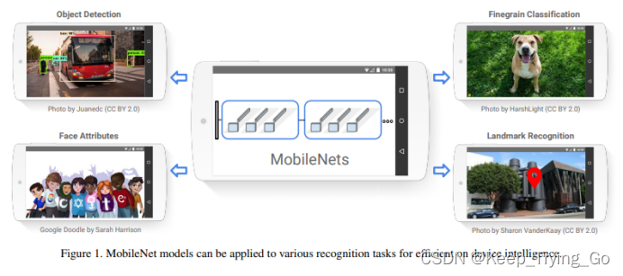
MobileNet是谷歌轻量化卷积神经网络，轻量化网络广泛用于无人驾驶，移动端，物联网的边缘计算和人工智能算法部署，所以MobileNet也成为了很多轻量化网络的骨干网络。
在这里插入图片描述

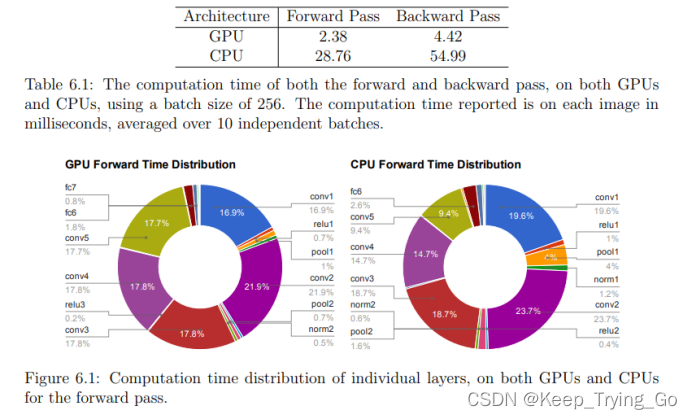
3.GPU和CPU上前向传播的计算量

在这里插入图片描述

https://www2.eecs.berkeley.edu/Pubs/TechRpts/2014/EECS-2014-93.pdf
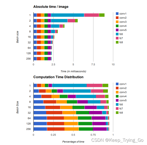
从上面的图表可以看出，随着batch size的大小不断增加，中间的卷积推理运算反而在不断的增加，而全连接层不断的减少，所以对于卷积过程的推理运算优化是很重要的。
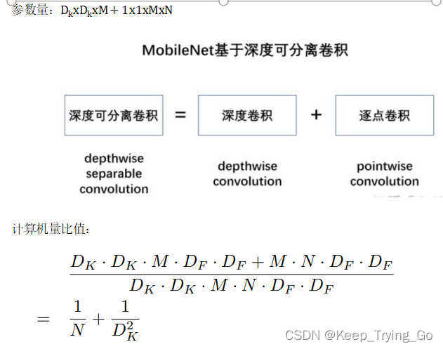
MobileNetV1减少基于深度卷积神经网络（depthwise separable convolutions）来进行优化的.

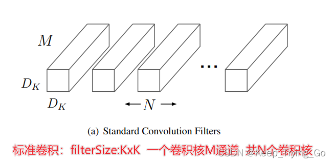
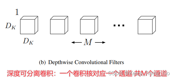
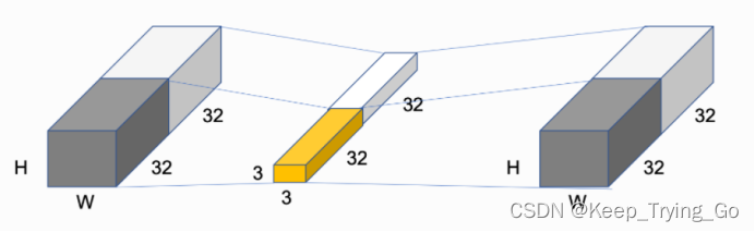
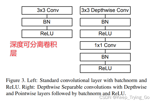
4.标准卷积和深度可分离卷积

参考博文：
https://mydreamambitious.blog.csdn.net/article/details/124503596
在这里插入图片描述

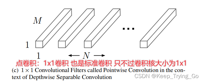
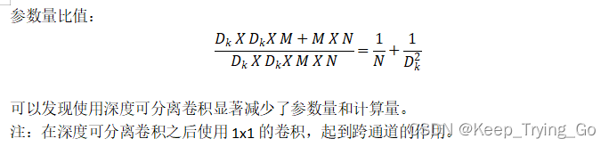
关于1x1卷积核的作用：https://mydreamambitious.blog.csdn.net/article/details/123027344
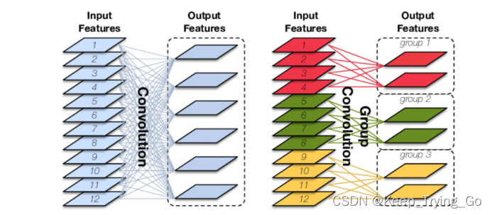
分组卷积：一个卷积只负责处理一部分feature map。

https://www.cnblogs.com/shine-lee/p/10243114.html

5.深度可分离卷积计算机量对比

在这里插入图片描述

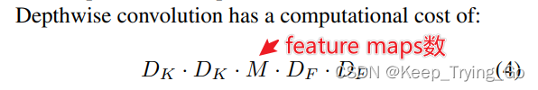
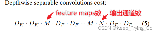
关于标准卷积，深度可分离卷积，分组卷积的参数量和计算机量的公式：
https://blog.csdn.net/qq_36758914/article/details/106885400

在这里插入图片描述
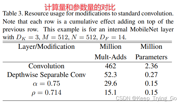
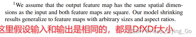
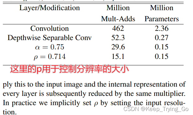
对于上面的计算量和参数计算：这里假设输入特征图大小：14x14x512；卷积核大小:3x3x512
（1）对于标准卷积：
参数量：3x3x512x512=235,293约等于2.36M
计算量：14x14x512x3x3x512=462,422,016约等于462M

（2）深度可分离卷积卷积：
参数量：3x3x512x14x14+512x512x14x14=52,283,392约等于52.3M
计算量：3x3x512+1x1x512x512=266,572约等于0.27M

（3）对于深度可分离卷积（α=0.75）卷积：
参数量：3x3x0.75x512+1x1x0.75x512x0.75x512=150,912约等于0.15M
计算量：3x3x0.75x512x14x14+0.75x512x0.75x512x14x14=29,578,752约等于29.6M

（4）对于深度可分离卷积（ρ=0.75）卷积：
参数量：3x3x0.75x512x0.714x14+0.75x512x0.75x512x0.714x14x0.714x14=15,079,129约等于15.1M
计算量：3x3x0.75x512+0.75x512x0.75x512=150,912约等于0.15M

6.MobileNetV1网络结构

在这里插入图片描述

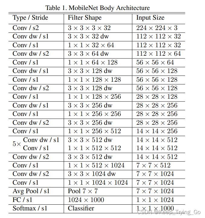
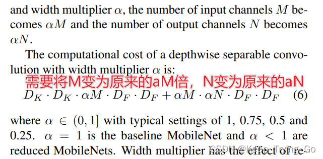
这个α等于1的时候不变，小于1的时候进行压缩；并且这个α可以被用于任何的模型结构。

7.结果的对比

在这里插入图片描述
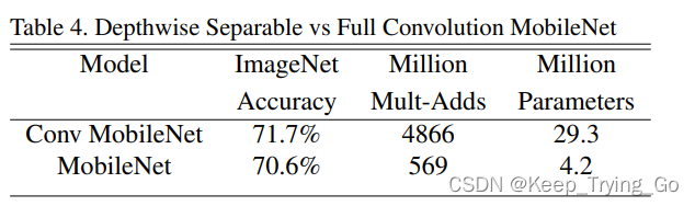
上面这张表表示了使用全卷积的MobileNet和使用深度可分离卷积的MobileNet在ImageNet上训练的结果，可以发现深度可分离卷积的MobileNet和全卷积的MobileNet在准确率上相差1.1个百分点，但是深度可分离卷积的MobileNet的计算量和参数量远远低于全卷积的MobileNet。所以使用深度可分离卷积的MobileNet是非常轻量化的。

在这里插入图片描述
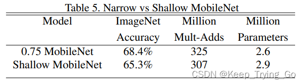
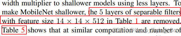
上面这张表表示了α=0.75的MobileNet和浅层的MobileNet准备率对比，发现浅层的MobileNet准确率下降较多，并且这里的计算量和参数量并没有太大的差别，所以深度的网络对于准确率的提升很重要。
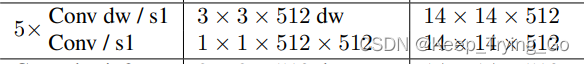
注：这里的浅层的MobileNet是指将网络中的去掉之后的结果。
在这里插入图片描述

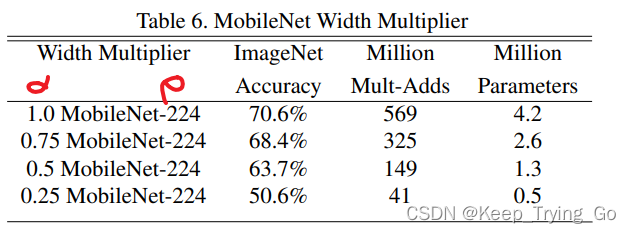
上面表示在相同的ρ（分辨率）的情况下，随着α的不断减小，准确率下降较多，虽然参数量和计算量也在不断的减少，可是这样做是不值得的。因为随着α不断的减小，卷积核的个数减少，权重减少，模型的表达能力也在不断降低，导致欠拟合。
在这里插入图片描述
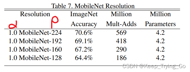
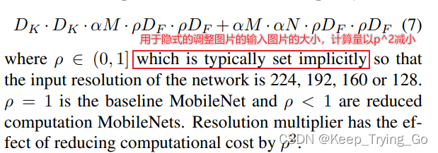
上面表示随着的ρ（分辨率）不断减小的情况下，α不变的情况下，准确率也下降了较多，虽然计算量也在不断的减少。

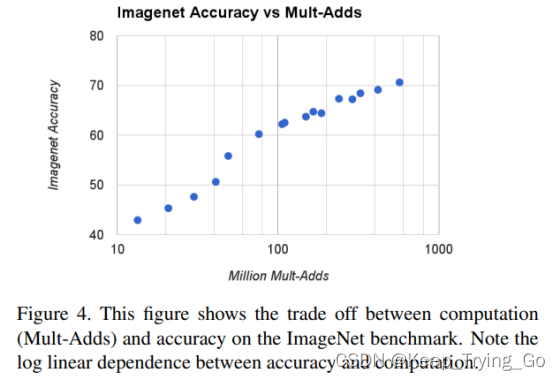
上面这张图表示了准确率随着计算量的增加而不断提高，并且是呈对数模型的增加，所以需要我们在准确率和计算量方面进行权衡。

在这里插入图片描述

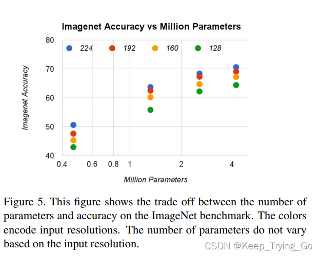
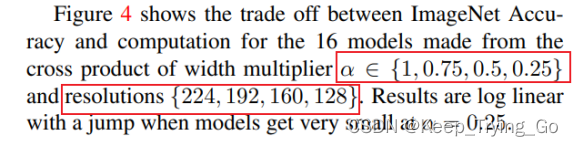
上面这个图表示了不同ρ（分辨率）和α（卷积核数）的16中组合准确率和计算量的权衡。
可以看到随着α的不断降低，准确率下降的更加快。

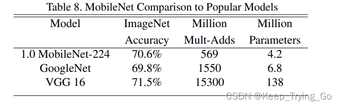
从上面的表中可以看到MobileNet准确率虽然比VGG16准确率较低，但是计算量和参数量是大大的降低。MobileNet的准确率又比GoogLeNet准确率要高。
在这里插入图片描述
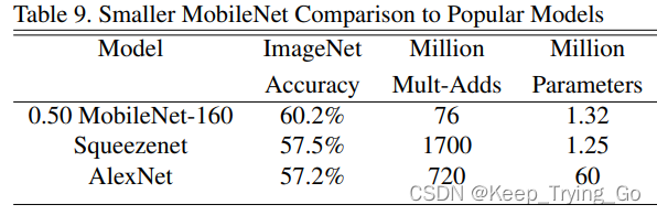
该表表示了MobileNet的准确率都比SqueezeNet和AlexNet的准确率都要高，而且参数量也是相对于他们要低很多。

8.MobileNetV1网络结构实现

import os
import keras
import numpy as np
import tensorflow as tf
from tensorflow.keras import layers

class DepthWiseConv(tf.keras.Model):
    def __init__(self,filter,stride=(1,1)):
        super(DepthWiseConv, self).__init__()
        self.depthwiseconv=layers.DepthwiseConv2D(kernel_size=[3,3],strides=stride,padding='same')
        self.depthbatch=layers.BatchNormalization()
        self.depthrelu=layers.Activation('relu')
        self.conv11=layers.Conv2D(filter,kernel_size=[1,1],strides=[1,1],padding='same')
        self.conv11batch=layers.BatchNormalization()
        self.conv11relu=layers.Activation('relu')
    def call(self,inputs,training=None):
        x=self.depthwiseconv(inputs)
        x=self.depthbatch(x)
        x=self.depthrelu(x)
        x=self.conv11(x)
        x=self.conv11batch(x)
        x=self.conv11relu(x)
        return x

class MobileNetV1(tf.keras.Model):
    def __init__(self,num_classes):
        super(MobileNetV1, self).__init__()
        self.conv1=layers.Conv2D(32,kernel_size=[3,3],strides=[2,2],padding='same')
        self.conv1batch=layers.BatchNormalization()
        self.conv1relu=layers.Activation('relu')
        self.depthconv=self.depthwiseconv()
        self.avgpool=layers.GlobalAveragePooling2D()
        self.dense=layers.Dense(num_classes)
        self.dropout=layers.Dropout(rate=0.5)
        self.softmax=layers.Activation('softmax')


    def depthwiseconv(self):
        depth=keras.Sequential([])
        depth.add(
            DepthWiseConv(filter=64,stride=(1,1))
        )
        depth.add(
            DepthWiseConv(filter=128, stride=(2, 2))
        )
        depth.add(
            DepthWiseConv(filter=128, stride=(1, 1))
        )
        depth.add(
            DepthWiseConv(filter=256, stride=(2, 2))
        )
        depth.add(
            DepthWiseConv(filter=256, stride=(1, 1))
        )
        depth.add(
            DepthWiseConv(filter=256, stride=(2, 2))
        )
        for i in range(5):
            depth.add(
                DepthWiseConv(filter=512, stride=(1, 1))
            )
        depth.add(
            DepthWiseConv(filter=512, stride=(2,2))
        )
        depth.add(
            DepthWiseConv(filter=1024, stride=(1, 1))
        )
        return depth
    def call(self,inputs,training=None):
        x=self.conv1(inputs)
        x=self.conv1batch(x)
        x=self.conv1relu(x)
        x=self.depthconv(x)
        x=self.avgpool(x)
        x=self.dense(x)
        x=self.dropout(x)
        x=self.softmax(x)

        return x

model_mobilenetv1=MobileNetV1(num_classes=1000)
model_mobilenetv1.build(input_shape=(None,224,224,3))
model_mobilenetv1.summary()


if __name__ == '__main__':
    print('pycharm')