Multiple Linear Regression(��Ԫ���Իع�)
֮ǰ��һƪ�����Իع������,��Ҹ���Ȥ���Կ�����ʹ��scikit-learnʵ�ּ����Իع�
Objectives(Ŀ��)
������ƪ����,����:1.ʹ��scikit-learnʵ�ֶ�Ԫ���Իع� 2.����һ��ģ��,ѵ����,������,��ʹ����
After completing this lab you will be able to:
- Use scikit-learn to implement Multiple Linear Regression
- Create a model, train it, test it and use the model
Table of contents
Importing Needed packages(������ذ�)
import matplotlib.pyplot as plt
import pandas as pd
import pylab as pl
import numpy as np
%matplotlib inline
Downloading Data(��������)
Understanding the Data(��������)
FuelConsumption.csv:
����������һ���ͺ����ݼ�, FuelConsumption.csv,���а����˼��ô������������������ض������ͺĵȼ����ƵĶ�����̼�ŷ�����
We have downloaded a fuel consumption dataset, FuelConsumption.csv, which contains model-specific fuel consumption ratings and estimated carbon dioxide emissions for new light-duty vehicles for retail sale in Canada. Dataset source
- MODELYEAR e.g. 2014
- MAKE e.g. Acura
- MODEL e.g. ILX
- VEHICLE CLASS e.g. SUV
- ENGINE SIZE e.g. 4.7
- CYLINDERS e.g 6
- TRANSMISSION e.g. A6
- FUELTYPE e.g. z
- FUEL CONSUMPTION in CITY(L/100 km) e.g. 9.9
- FUEL CONSUMPTION in HWY (L/100 km) e.g. 8.9
- FUEL CONSUMPTION COMB (L/100 km) e.g. 9.2
- CO2 EMISSIONS (g/km) e.g. 182 --> low --> 0
Reading the data in(��ȡ����)
# df = pd.read_csv("FuelConsumption.csv")
df=pd.read_csv("D:\MLwithPython\FuelConsumptionCo2.csv")
# take a look at the dataset
df.head()
| MODELYEAR | MAKE | MODEL | VEHICLECLASS | ENGINESIZE | CYLINDERS | TRANSMISSION | FUELTYPE | FUELCONSUMPTION_CITY | FUELCONSUMPTION_HWY | FUELCONSUMPTION_COMB | FUELCONSUMPTION_COMB_MPG | CO2EMISSIONS | |
|---|---|---|---|---|---|---|---|---|---|---|---|---|---|
| 0 | 2014 | ACURA | ILX | COMPACT | 2.0 | 4 | AS5 | Z | 9.9 | 6.7 | 8.5 | 33 | 196 |
| 1 | 2014 | ACURA | ILX | COMPACT | 2.4 | 4 | M6 | Z | 11.2 | 7.7 | 9.6 | 29 | 221 |
| 2 | 2014 | ACURA | ILX HYBRID | COMPACT | 1.5 | 4 | AV7 | Z | 6.0 | 5.8 | 5.9 | 48 | 136 |
| 3 | 2014 | ACURA | MDX 4WD | SUV - SMALL | 3.5 | 6 | AS6 | Z | 12.7 | 9.1 | 11.1 | 25 | 255 |
| 4 | 2014 | ACURA | RDX AWD | SUV - SMALL | 3.5 | 6 | AS6 | Z | 12.1 | 8.7 | 10.6 | 27 | 244 |
��������ѡ������ȥ���ع����
Let��s select some features that we want to use for regression.
cdf = df[['ENGINESIZE','CYLINDERS','FUELCONSUMPTION_CITY','FUELCONSUMPTION_HWY','FUELCONSUMPTION_COMB','CO2EMISSIONS']]
cdf.head(9)
| ENGINESIZE | CYLINDERS | FUELCONSUMPTION_CITY | FUELCONSUMPTION_HWY | FUELCONSUMPTION_COMB | CO2EMISSIONS | |
|---|---|---|---|---|---|---|
| 0 | 2.0 | 4 | 9.9 | 6.7 | 8.5 | 196 |
| 1 | 2.4 | 4 | 11.2 | 7.7 | 9.6 | 221 |
| 2 | 1.5 | 4 | 6.0 | 5.8 | 5.9 | 136 |
| 3 | 3.5 | 6 | 12.7 | 9.1 | 11.1 | 255 |
| 4 | 3.5 | 6 | 12.1 | 8.7 | 10.6 | 244 |
| 5 | 3.5 | 6 | 11.9 | 7.7 | 10.0 | 230 |
| 6 | 3.5 | 6 | 11.8 | 8.1 | 10.1 | 232 |
| 7 | 3.7 | 6 | 12.8 | 9.0 | 11.1 | 255 |
| 8 | 3.7 | 6 | 13.4 | 9.5 | 11.6 | 267 |
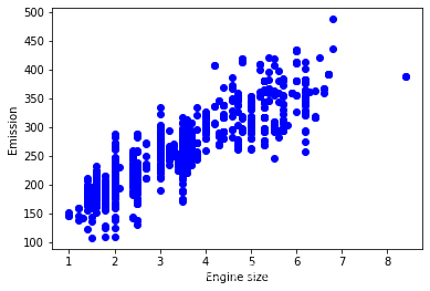
��һ��Emission��Engine Size֮��Ĺ�ϵ
Let��s plot Emission values with respect to Engine size:
plt.scatter(cdf.ENGINESIZE, cdf.CO2EMISSIONS,  color='blue')
plt.xlabel("Engine size")
plt.ylabel("Emission")
plt.show()

Creating train and test dataset(����ѵ�����Ͳ��Լ�)
ѵ��/���Էָ��漰�����ݼ��ָ�Ϊ�����ѵ�����Ͳ��Լ��� ֮��,ʹ��ѵ��������ѵ��,ʹ�ò��Լ����в��ԡ�
Train/Test Split involves splitting the dataset into training and testing sets that are mutually exclusive. After which, you train with the training set and test with the testing set.
�⽫���������ȷ���ṩ��ȷ������,��Ϊ�������ݼ���������ѵ��ģ�͵����ݼ���һ���֡� ���,�������Ǹ��õ��������ǵ�ģ�����������ϵķ��������
This will provide a more accurate evaluation on out-of-sample accuracy because the testing dataset is not part of the dataset that have been used to train the model. Therefore, it gives us a better understanding of how well our model generalizes on new data.
����ζ������֪���������ݼ���ÿ�����ݵ�Ľ��,��ʹ�����dz��ʺ����ڲ���! ������Щ����û�б�����ѵ��ģ��,����ģ�Ͳ�֪����Щ���ݵ�Ľ���� ���,�ӱ����Ͻ�,������������������ԡ�
This means that we know the outcome of each data point in the testing dataset, making it great to test with! Since this data has not been used to train the model, the model has no knowledge of the outcome of these data points. So, in essence, it is truly an out-of-sample testing.
�����ǽ����ݼ��ֳ�ѵ�����Ͳ��Լ��� �������ݼ���80%������ѵ��,20%���ڲ��ԡ� ����ʹ��**np.random.rand()**��������һ��������ѡ�������:
Let��s split our dataset into train and test sets. 80% of the entire dataset will be used for training and 20% for testing. We create a mask to select random rows using np.random.rand() function:
msk = np.random.rand(len(df)) < 0.8
train = cdf[msk]
test = cdf[~msk]
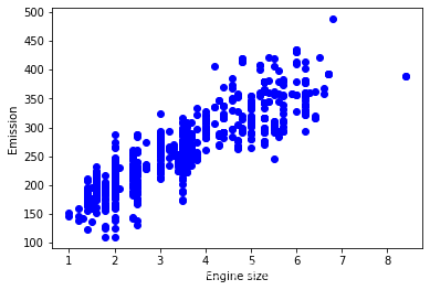
Train data distribution(���ݵķֲ�)
plt.scatter(train.ENGINESIZE, train.CO2EMISSIONS,  color='blue')
plt.xlabel("Engine size")
plt.ylabel("Emission")
plt.show()

Multiple Regression Model
��ʵ��,Ӱ�������̼�ŷŵ������кܶࡣ ���ж���Ա���ʱ,������̳�Ϊ��Ԫ���Իع顣 ��Ԫ���Իع��һ������������������FUELCONSUMPTION_COMB��EngineSize��Cylinders��������Ԥ�������̼�ŷš� ����ĺô��Ƕ�Ԫ���Իع�ģ���Ǽ����Իع�ģ�͵���չ��
In reality, there are multiple variables that impact the co2emission. When more than one independent variable is present, the process is called multiple linear regression. An example of multiple linear regression is predicting co2emission using the features FUELCONSUMPTION_COMB, EngineSize and Cylinders of cars. The good thing here is that multiple linear regression model is the extension of the simple linear regression model.
from sklearn import linear_model
regr = linear_model.LinearRegression()
x = np.asanyarray(train[['ENGINESIZE','CYLINDERS','FUELCONSUMPTION_COMB']])
y = np.asanyarray(train[['CO2EMISSIONS']])
regr.fit (x, y)
# The coefficients
print ('Coefficients: ', regr.coef_)
Coefficients: [[11.71513251 7.04363114 9.5232153 ]]
��ǰ����,ϵ�����ؾ������ֱ�ߵIJ�����
As mentioned before, Coefficient and Intercept are the parameters of the fitted line.
��������һ������3�������Ķ�Ԫ���Իع�ģ��,����Ϊ��ƽ��Ľؾ��ϵ��,sklearn���Դ����ǵ������й������ǡ� Scikit-learnʹ����ͨ����ͨ��С���˷������������⡣
Given that it is a multiple linear regression model with 3 parameters and that the parameters are the intercept and coefficients of the hyperplane, sklearn can estimate them from our data. Scikit-learn uses plain Ordinary Least Squares method to solve this problem.
Ordinary Least Squares (OLS)(��С���˷��C���о�ѧ��)
OLS��һ�ֹ������Իع�ģ����δ֪�����ķ����� OLSͨ����С��Ŀ������������Ժ���Ԥ��ֵ֮���ƽ������ѡ��һ����ͱ��������Ժ����IJ����� ���仰˵,����ͼ��С�����ݼ�������������Ŀ�����(y)�����ǵ�Ԥ�����(
y
^
\hat{y}
y^?)֮���ƽ�����(SSE)��������(MSE)���ܺ͡�
OLS is a method for estimating the unknown parameters in a linear regression model. OLS chooses the parameters of a linear function of a set of explanatory variables by minimizing the sum of the squares of the differences between the target dependent variable and those predicted by the linear function. In other words, it tries to minimizes the sum of squared errors (SSE) or mean squared error (MSE) between the target variable (y) and our predicted output (
y
^
\hat{y}
y^?) over all samples in the dataset.
OLS����ͨ�����·����ҵ���Ѳ���:
OLS can find the best parameters using of the following methods:
- Solving the model parameters analytically using closed-form equations
- Using an optimization algorithm (Gradient Descent, Stochastic Gradient Descent, Newton��s Method, etc.)
Prediction(Ԥ��)
y_hat= regr.predict(test[['ENGINESIZE','CYLINDERS','FUELCONSUMPTION_COMB']])
x = np.asanyarray(test[['ENGINESIZE','CYLINDERS','FUELCONSUMPTION_COMB']])
y = np.asanyarray(test[['CO2EMISSIONS']])
print("Residual sum of squares: %.2f"
      % np.mean((y_hat - y) ** 2))

# Explained variance score: 1 is perfect prediction
print('Variance score: %.2f' % regr.score(x, y))
Residual sum of squares: 538.19
Variance score: 0.85
Explained variance regression score:
Let
y
^
\hat{y}
y^? be the estimated target output, y the corresponding (correct) target output, and Var be the Variance (the square of the standard deviation). Then the explained variance is estimated as follows:
explainedVariance
(
y
,
y
^
)
=
1
?
V
a
r
y
?
y
^
V
a
r
y
\texttt{explainedVariance}(y, \hat{y}) = 1 - \frac{Var{ y - \hat{y}}}{Var{y}}
explainedVariance(y,y^?)=1?VaryVary?y^??
The best possible score is 1.0, the lower values are worse.(Խ�ӽ���1Խ��)
Practice(��ϰ)
Try to use a multiple linear regression with the same dataset, but this time use FUELCONSUMPTION_CITY and FUELCONSUMPTION_HWY instead of FUELCONSUMPTION_COMB. Does it result in better accuracy?# write your code here
regr = linear_model.LinearRegression()
x = np.asanyarray(train[['ENGINESIZE','CYLINDERS','FUELCONSUMPTION_CITY','FUELCONSUMPTION_HWY']])
y = np.asanyarray(train[['CO2EMISSIONS']])
regr.fit (x, y)
# The coefficients
print ('Coefficients: ', regr.coef_)
# Ԥ��
y_hat= regr.predict(test[['ENGINESIZE','CYLINDERS','FUELCONSUMPTION_CITY','FUELCONSUMPTION_HWY']])
x = np.asanyarray(test[['ENGINESIZE','CYLINDERS','FUELCONSUMPTION_CITY','FUELCONSUMPTION_HWY']])
y = np.asanyarray(test[['CO2EMISSIONS']])
print("Residual sum of squares: %.2f"
% np.mean((y_hat - y) ** 2))
# Explained variance score: 1 is perfect prediction
print('Variance score: %.2f' % regr.score(x, y))
Coefficients:  [[11.77637455  6.7350317   5.99648967  3.30209632]]
Residual sum of squares: 537.85
Variance score: 0.85