[人工智能]第4周学习：MobileNetV1 V2 V3

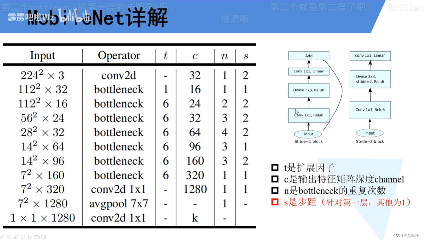
MobileNet V1 & V2

传统卷积神经网络内存需求大、运算量大，导致无法在移动设备以及嵌入式设备上运行。MobileNet网络由google团队在2017年提出，专注于移动端或者嵌入式设备中的轻量级CNN网络。相比传统卷积神经网络，在准确率小幅降低的前提下大大减少模型参数与运算量，并且增加了两个超参数，α用于控制卷积层卷积核个数，β用于控制输入图像大小。


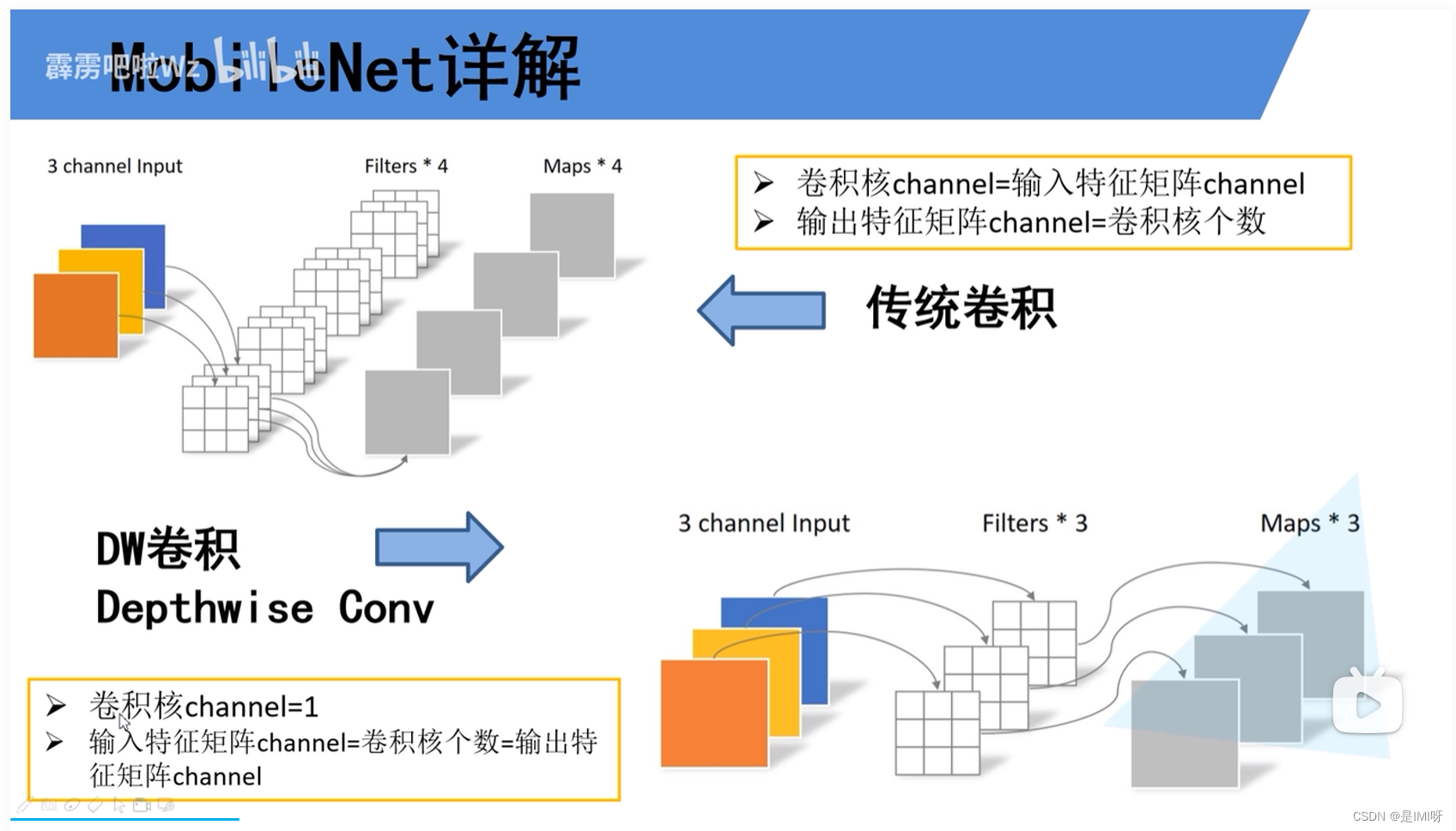
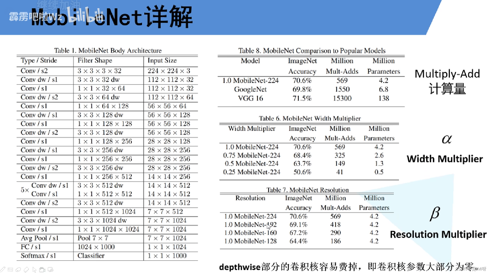
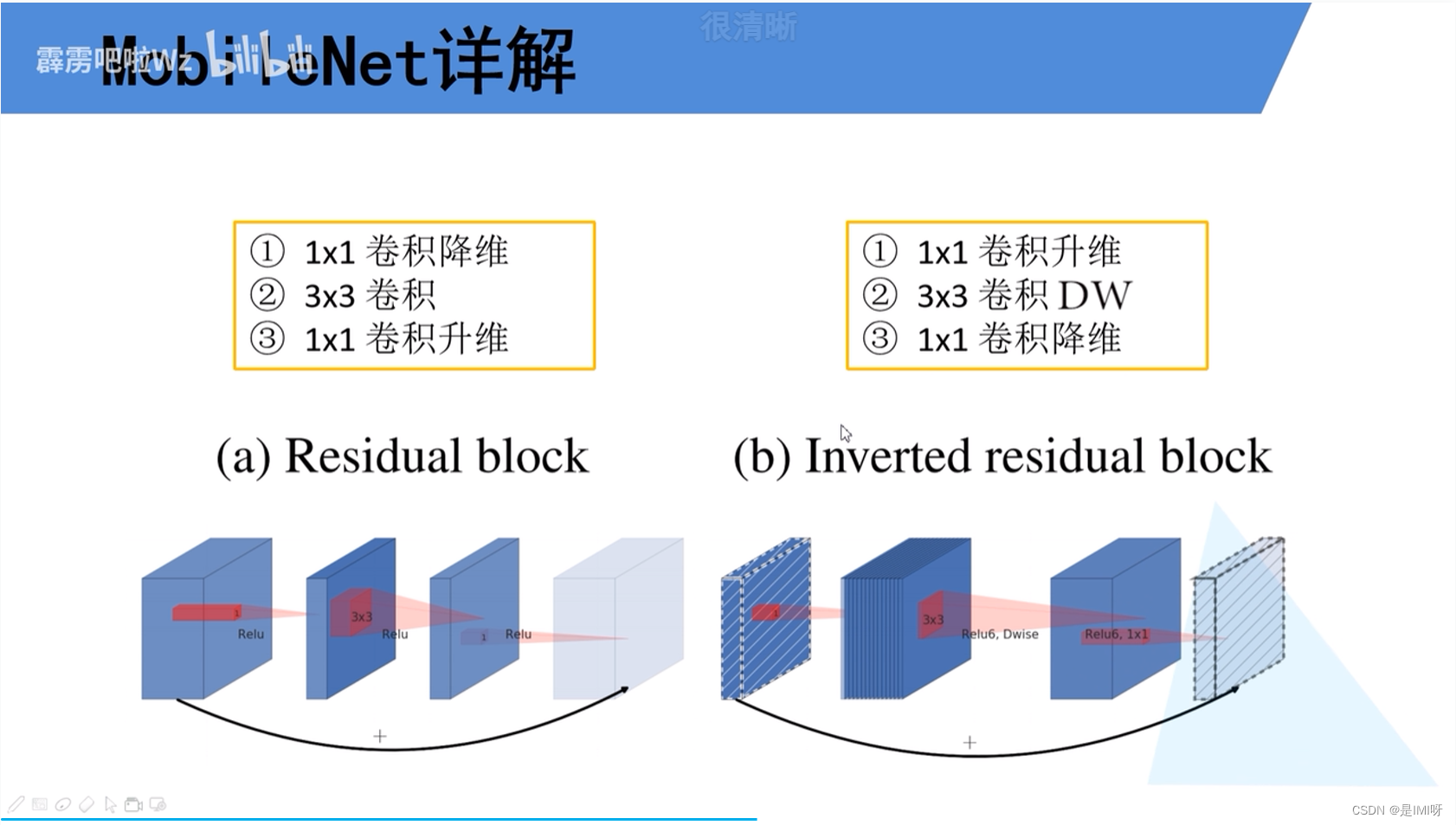
MobileNet V1缺点：depthwise部分的卷积核容易费掉，即卷积核参数大部分为零。，因此引入MobileNet V2网络。相比V1而言，V2准确率更高，模型更小。亮点是引入Inverted Residuals倒残差结构和Linear Bottlenecks。

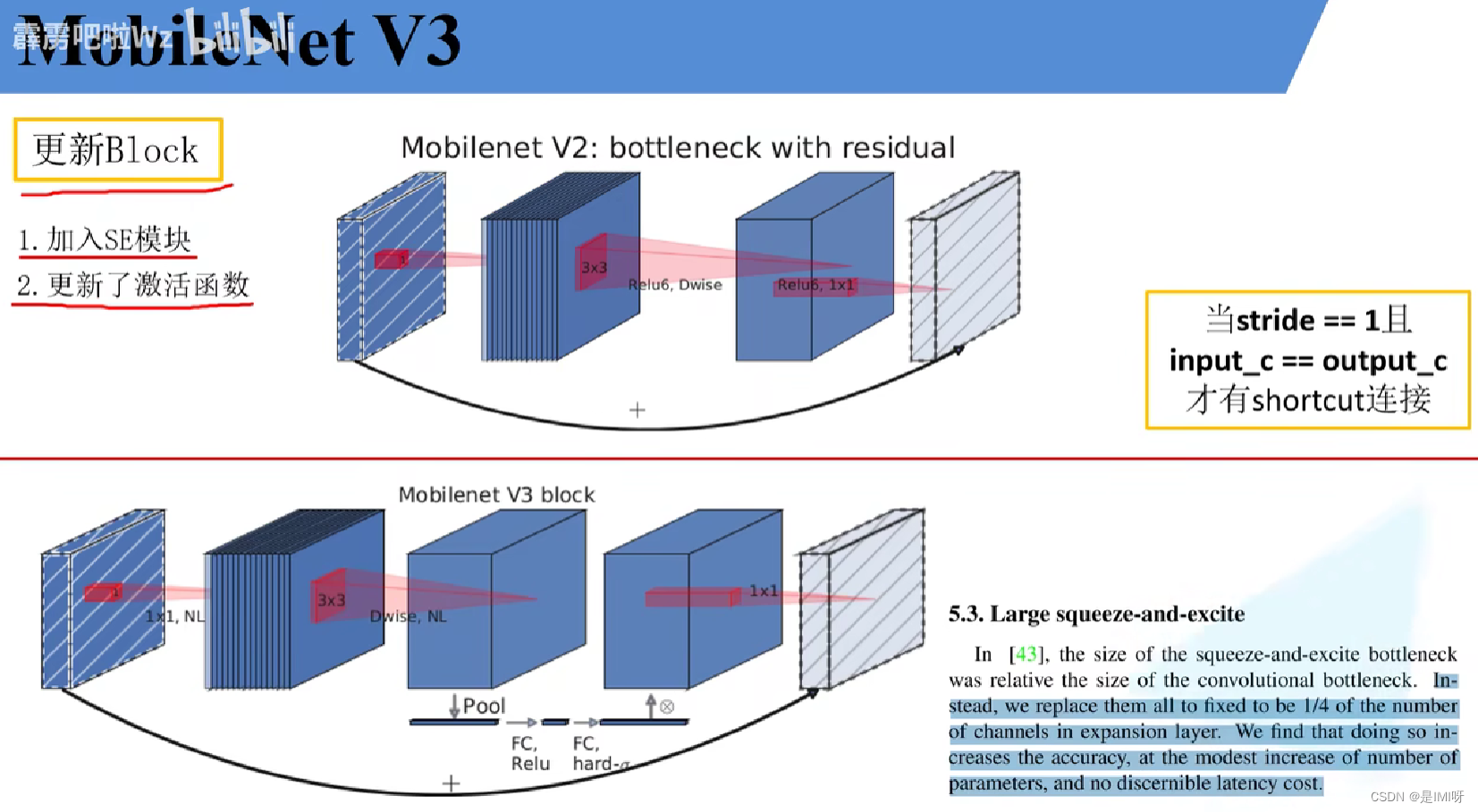
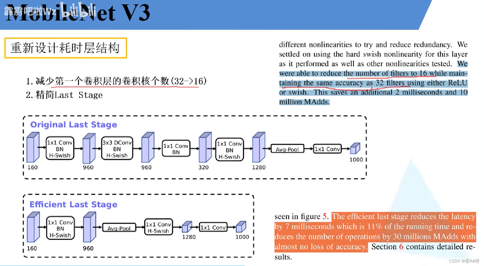
MobileNet V3

更新了Block(bneck)，使用NAS搜索参数(Neural Architecture Search)，重新设计耗时层结构

SENet 的基本原理和代码

卷积核是卷积神经网络的核心，通常被看作是在局部感受野上，将空间上的信息和特征维度上的信息进行聚合的信息聚合体。卷积神经网络由一系列卷积层、非线性层和下采样层构成，这样它们能够从全局感受野上去捕获图像的特征来进行图像的描述。SENet即为Squeeze-and-Excitation Networks，主要有两个重要操作Squeeze和Excitation。下图是SE模块的示意图。

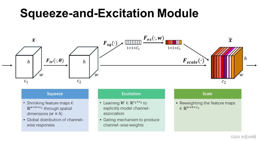
首先是Squeeze 操作，我们顺着空间维度来进行特征压缩，将每个二维的特征通道变成一个实数，这个实数某种程度上具有全局的感受野，并且输出的维度和输入的特征通道数相匹配。它表征着在特征通道上响应的全局分布，而且使得靠近输入的层也可以获得全局的感受野。其次是Excitation 操作，它是一个类似于循环神经网络中门的机制。通过参数来为每个特征通道生成权重，其中参数被学习用来显式地建模特征通道间的相关性。最后是一个Reweight的操作，我们将Excitation的输出的权重看做是进过特征选择后的每个特征通道的重要性，然后通过乘法逐通道加权到先前的特征上，完成在通道维度上的对原始特征的重标定。最后是一个Reweight的操作，我们将Excitation的输出的权重看做是进过特征选择后的每个特征通道的重要性，然后通过乘法逐通道加权到先前的特征上，完成在通道维度上的对原始特征的重标定。

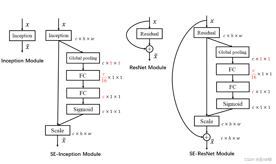
上左图是将SE模块嵌入到Inception结构的一个示例。方框旁边的维度信息代表该层的输出。这里我们使用global average pooling 作为Squeeze 操作。紧接着两个Fully Connected 层组成一个Bottleneck结构去建模通道间的相关性，并输出和输入特征同样数目的权重。我们首先将特征维度降低到输入的1/16 ，然后经过ReLu激活后再通过一个Fully Connected 层升回到原来的维度。 这样做比直接用一个Fully Connected 层的好处在于：1）具有更多的非线性，可以更好地拟合通道间复杂的相关性；2）极大地减少了参数量和计算量。然后通过一个Sigmoid的门获得0~1之间归一化的权重，最后通过一个Scale的操作来将归一化后的权重加权到每个通道的特征上。
从上面的介绍中可以发现，SENet构造非常简单，而且很容易被部署，不需要引入新的函数或者层。除此之外，它还在模型和计算复杂度上具有良好的特性。

HybridSN 高光谱分类-代码练习

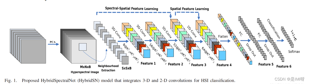
通常，HybridSN是频谱空间3-D CNN，然后是空间2-D-CNN。论文中提到，仅使用2-D-CNN或3-D-CNN有一些缺点，例如缺少频道关系信息或模型非常复杂。这也阻止了这些方法在HSI空间上获得更高的准确性。主要原因是由于HSI是体积数据，也有光谱维度。单独的2-D-CNN无法从光谱维度上提取良好的区分特征，同样，深 3-D-CNN的计算更加复杂，而论文中提出的HybridSN模型，克服了先前模型的这些缺点。3-D-CNN和2-D-CNN层以推荐的模型组装成合适的网络，充分利用光谱图和空间特征图，最大限度地提高精度。
论文中使用了2D、3D卷积，可以看出的是3D卷积明显多一个维度，对应的激活函数也多一个维度。此外，2D conv的卷积核其实是(c, k_h, k_w)，3D conv的卷积核就是(c, k_d, k_h, k_w)，其中k_d就是多出来的第三维，根据具体应用，在视频中就是时间维，在CT图像中就是层数维。
并且，论文中先进行三维卷积，再进行二维卷积，这说明它们适用的场景不同，我们容易减少数据集的维度，但不容易增加数据集维度，所以应当先进行高维的卷积。另外，三维卷积产生的参数比二维卷积要少得多。

网络搭建参考高光谱图像分类 HybridSN，实现如下：
Step 1：取得数据，引入基本函数库

! wget http://www.ehu.eus/ccwintco/uploads/6/67/Indian_pines_corrected.mat
! wget http://www.ehu.eus/ccwintco/uploads/c/c4/Indian_pines_gt.mat
! pip install spectral

import numpy as np
import matplotlib.pyplot as plt
import scipy.io as sio
from sklearn.decomposition import PCA
from sklearn.model_selection import train_test_split
from sklearn.metrics import confusion_matrix, accuracy_score, classification_report, cohen_kappa_score
import spectral
import torch
import torchvision
import torch.nn as nn
import torch.nn.functional as F
import torch.optim as optim

Step 2：定义HybridSN类模块

class_num = 16
windowSize = 25
K = 30        #参考Hybrid-Spectral-Net
rate = 16	

class HybridSN(nn.Module):
 #定义各个层的部分
  def __init__(self):
    super(HybridSN, self).__init__()
    self.S = windowSize
    self.L = K;

    #self.conv_block = nn.Sequential()
    ## convolutional layers
    self.conv1 = nn.Conv3d(in_channels=1, out_channels=8, kernel_size=(7, 3, 3))
    self.conv2 = nn.Conv3d(in_channels=8, out_channels=16, kernel_size=(5, 3, 3))
    self.conv3 = nn.Conv3d(in_channels=16, out_channels=32, kernel_size=(3, 3, 3))
    
    #不懂 inputX经过三重3d卷积的大小
    inputX = self.get2Dinput()
    inputConv4 = inputX.shape[1] * inputX.shape[2]
    # conv4 （24*24=576, 19, 19），64个 3x3 的卷积核 ==>（（64, 17, 17）
    self.conv4 = nn.Conv2d(inputConv4, 64, kernel_size=(3, 3))

    #self-attention
    self.sa1 = nn.Conv2d(64, 64//rate, kernel_size=1)
    self.sa2 = nn.Conv2d(64//rate, 64, kernel_size=1)
    
    # 全连接层（256个节点） # 64 * 17 * 17 = 18496
    self.dense1 = nn.Linear(18496, 256) 
    # 全连接层（128个节点）
    self.dense2 = nn.Linear(256, 128)
    # 最终输出层(16个节点)
    self.dense3 = nn.Linear(128, class_num)
    
    #让某个神经元的激活值以一定的概率p，让其停止工作，这次训练过程中不更新权值，也不参加神经网络的计算。
    #但是它的权重得保留下来，可用于下次工作
    self.drop = nn.Dropout(p = 0.4)
    self.soft = nn.Softmax(dim=1)
    pass

  #辅助函数，求经历过三重卷积后二维的一个大小
  def get2Dinput(self):
    #torch.no_grad(): 做运算，但不计入梯度记录
    with torch.no_grad():
      x = torch.zeros((1, 1, self.L, self.S, self.S))
      x = self.conv1(x)
      x = self.conv2(x)
      x = self.conv3(x)
    return x
    pass

  #必须重载的部分，X代表输入
  def forward(self, x):
    #F在上文有定义torch.nn.functional，是已定义好的一组名称
    out = F.relu(self.conv1(x))
    out = F.relu(self.conv2(out))
    out = F.relu(self.conv3(out))

    # 进行二维卷积，因此把前面的 32*18 reshape 一下，得到 （576, 19, 19）
    out = out.view(-1, out.shape[1] * out.shape[2], out.shape[3], out.shape[4])
    out = F.relu(self.conv4(out))

    # Squeeze 第三维卷成1了
    weight = F.avg_pool2d(out, out.size(2))    #参数为输入，kernel
    # Excitation: sa（压缩到16分之一）--Relu--fc（激到之前维度）--Sigmoid（保证输出为0至1之间）
    weight = F.relu(self.sa1(weight))
    weight = F.sigmoid(self.sa2(weight))
    out = out * weight

    # flatten: 变为 18496 维的向量，
    out = out.view(out.size(0), -1)

    out = F.relu(self.dense1(out))
    out = self.drop(out)
    out = F.relu(self.dense2(out))
    out = self.drop(out)
    out = self.dense3(out)
    return out
    pass
# 随机输入，测试网络结构是否通
# x = torch.randn(1, 1, 30, 25, 25)
# net = HybridSN()
# y = net(x)
# print(y.shape)

Step 3：定义HybridSN类模块
首先对高光谱数据实施PCA降维，然后创建 keras 方便处理的数据格式，随机抽取 10% 数据做为训练集，剩余的做为测试集。四个函数分别进行主成分分析、零填充、创建patch和划分数据集。

# 对高光谱数据 X 应用 PCA 变换
def applyPCA(X, numComponents):
    newX = np.reshape(X, (-1, X.shape[2]))
    pca = PCA(n_components=numComponents, whiten=True)
    newX = pca.fit_transform(newX)
    newX = np.reshape(newX, (X.shape[0], X.shape[1], numComponents))
    return newX

# 对单个像素周围提取 patch 时，边缘像素就无法取了，因此，给这部分像素进行 padding 操作
def padWithZeros(X, margin=2):
    newX = np.zeros((X.shape[0] + 2 * margin, X.shape[1] + 2* margin, X.shape[2]))
    x_offset = margin
    y_offset = margin
    newX[x_offset:X.shape[0] + x_offset, y_offset:X.shape[1] + y_offset, :] = X
    return newX

# 在每个像素周围提取 patch ，然后创建成符合 keras 处理的格式
def createImageCubes(X, y, windowSize=5, removeZeroLabels = True):
    # 给 X 做 padding
    margin = int((windowSize - 1) / 2)
    zeroPaddedX = padWithZeros(X, margin=margin)
    # split patches
    patchesData = np.zeros((X.shape[0] * X.shape[1], windowSize, windowSize, X.shape[2]))
    patchesLabels = np.zeros((X.shape[0] * X.shape[1]))
    patchIndex = 0
    for r in range(margin, zeroPaddedX.shape[0] - margin):
        for c in range(margin, zeroPaddedX.shape[1] - margin):
            patch = zeroPaddedX[r - margin:r + margin + 1, c - margin:c + margin + 1]   
            patchesData[patchIndex, :, :, :] = patch
            patchesLabels[patchIndex] = y[r-margin, c-margin]
            patchIndex = patchIndex + 1
    if removeZeroLabels:
        patchesData = patchesData[patchesLabels>0,:,:,:]
        patchesLabels = patchesLabels[patchesLabels>0]
        patchesLabels -= 1
    return patchesData, patchesLabels

def splitTrainTestSet(X, y, testRatio, randomState=345):
    X_train, X_test, y_train, y_test = train_test_split(X, y, test_size=testRatio, random_state=randomState, stratify=y)
    return X_train, X_test, y_train, y_test

Step 4：读取并创建数据集

# 地物类别
class_num = 16
X = sio.loadmat('Indian_pines_corrected.mat')['indian_pines_corrected']
y = sio.loadmat('Indian_pines_gt.mat')['indian_pines_gt']

# 用于测试样本的比例
test_ratio = 0.90
# 每个像素周围提取 patch 的尺寸
patch_size = 25
# 使用 PCA 降维，得到主成分的数量
pca_components = 30

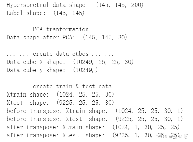
print('Hyperspectral data shape: ', X.shape)
print('Label shape: ', y.shape)

print('\n... ... PCA tranformation ... ...')
X_pca = applyPCA(X, numComponents=pca_components)
print('Data shape after PCA: ', X_pca.shape)

print('\n... ... create data cubes ... ...')
X_pca, y = createImageCubes(X_pca, y, windowSize=patch_size)
print('Data cube X shape: ', X_pca.shape)
print('Data cube y shape: ', y.shape)

print('\n... ... create train & test data ... ...')
Xtrain, Xtest, ytrain, ytest = splitTrainTestSet(X_pca, y, test_ratio)
print('Xtrain shape: ', Xtrain.shape)
print('Xtest  shape: ', Xtest.shape)

# 改变 Xtrain, Ytrain 的形状，以符合 keras 的要求
Xtrain = Xtrain.reshape(-1, patch_size, patch_size, pca_components, 1)
Xtest  = Xtest.reshape(-1, patch_size, patch_size, pca_components, 1)
print('before transpose: Xtrain shape: ', Xtrain.shape) 
print('before transpose: Xtest  shape: ', Xtest.shape) 

# 为了适应 pytorch 结构，数据要做 transpose
Xtrain = Xtrain.transpose(0, 4, 3, 1, 2)
Xtest  = Xtest.transpose(0, 4, 3, 1, 2)
print('after transpose: Xtrain shape: ', Xtrain.shape) 
print('after transpose: Xtest  shape: ', Xtest.shape) 


""" Training dataset"""
class TrainDS(torch.utils.data.Dataset): 
    def __init__(self):
        self.len = Xtrain.shape[0]
        self.x_data = torch.FloatTensor(Xtrain)
        self.y_data = torch.LongTensor(ytrain)        
    def __getitem__(self, index):
        # 根据索引返回数据和对应的标签
        return self.x_data[index], self.y_data[index]
    def __len__(self): 
        # 返回文件数据的数目
        return self.len

""" Testing dataset"""
class TestDS(torch.utils.data.Dataset): 
    def __init__(self):
        self.len = Xtest.shape[0]
        self.x_data = torch.FloatTensor(Xtest)
        self.y_data = torch.LongTensor(ytest)
    def __getitem__(self, index):
        # 根据索引返回数据和对应的标签
        return self.x_data[index], self.y_data[index]
    def __len__(self): 
        # 返回文件数据的数目
        return self.len

# 创建 trainloader 和 testloader
trainset = TrainDS()
testset  = TestDS()
train_loader = torch.utils.data.DataLoader(dataset=trainset, batch_size=128, shuffle=True, num_workers=2)

Step 5：模型训练

# 使用GPU训练，可以在菜单 "代码执行工具" -> "更改运行时类型" 里进行设置
device = torch.device("cuda:0" if torch.cuda.is_available() else "cpu")

# 网络放到GPU上
net = HybridSN().to(device)
criterion = nn.CrossEntropyLoss()
optimizer = optim.Adam(net.parameters(), lr=0.001)

# 开始训练
total_loss = 0
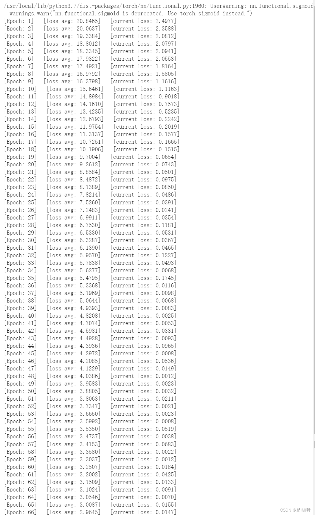
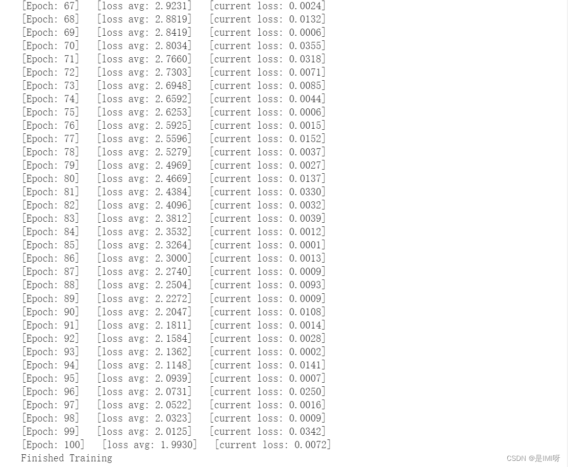
for epoch in range(100):
    for i, (inputs, labels) in enumerate(train_loader):
        inputs = inputs.to(device)
        labels = labels.to(device)
        # 优化器梯度归零
        optimizer.zero_grad()
        # 正向传播 +　反向传播 + 优化 
        outputs = net(inputs)
        loss = criterion(outputs, labels)
        loss.backward()
        optimizer.step()
        total_loss += loss.item()
    print('[Epoch: %d]   [loss avg: %.4f]   [current loss: %.4f]' %(epoch + 1, total_loss/(epoch+1), loss.item()))

print('Finished Training')

Step 6：模型测试

count = 0
# 模型测试
for inputs, _ in test_loader:
    inputs = inputs.to(device)
    outputs = net(inputs)
    outputs = np.argmax(outputs.detach().cpu().numpy(), axis=1)
    if count == 0:
        y_pred_test =  outputs
        count = 1
    else:
        y_pred_test = np.concatenate( (y_pred_test, outputs) )

# 生成分类报告
classification = classification_report(ytest, y_pred_test, digits=4)
print(classification)

第一次测试结果：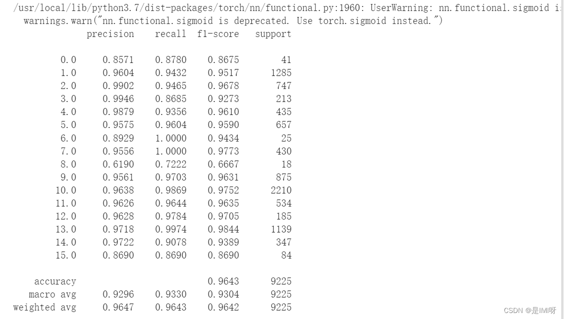
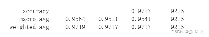
第二次测试结果：

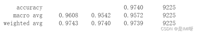
第三次测试结果：

Step 7：显示分类结果

from operator import truediv
#计算各个类准确率
def AA_andEachClassAccuracy(confusion_matrix):
    counter = confusion_matrix.shape[0]
    list_diag = np.diag(confusion_matrix)
    list_raw_sum = np.sum(confusion_matrix, axis=1)
    each_acc = np.nan_to_num(truediv(list_diag, list_raw_sum))
    average_acc = np.mean(each_acc)
    return each_acc, average_acc


def reports (test_loader, y_test, name):
    count = 0
    for inputs, _ in test_loader:
        inputs = inputs.to(device)
        outputs = net(inputs)
        outputs = np.argmax(outputs.detach().cpu().numpy(), axis=1)
        if count == 0:
            y_pred =  outputs
            count = 1
        else:
            y_pred = np.concatenate( (y_pred, outputs) )
#选择不同类型的数据集，在结果文件中做以下说明
    if name == 'IP':
        target_names = ['Alfalfa', 'Corn-notill', 'Corn-mintill', 'Corn'
                        ,'Grass-pasture', 'Grass-trees', 'Grass-pasture-mowed', 
                        'Hay-windrowed', 'Oats', 'Soybean-notill', 'Soybean-mintill',
                        'Soybean-clean', 'Wheat', 'Woods', 'Buildings-Grass-Trees-Drives',
                        'Stone-Steel-Towers']
    elif name == 'SA':
        target_names = ['Brocoli_green_weeds_1','Brocoli_green_weeds_2','Fallow','Fallow_rough_plow','Fallow_smooth',
                        'Stubble','Celery','Grapes_untrained','Soil_vinyard_develop','Corn_senesced_green_weeds',
                        'Lettuce_romaine_4wk','Lettuce_romaine_5wk','Lettuce_romaine_6wk','Lettuce_romaine_7wk',
                        'Vinyard_untrained','Vinyard_vertical_trellis']
    elif name == 'PU':
        target_names = ['Asphalt','Meadows','Gravel','Trees', 'Painted metal sheets','Bare Soil','Bitumen',
                        'Self-Blocking Bricks','Shadows']
    
    classification = classification_report(y_test, y_pred, target_names=target_names)
    oa = accuracy_score(y_test, y_pred)
    confusion = confusion_matrix(y_test, y_pred)
    each_acc, aa = AA_andEachClassAccuracy(confusion)
    kappa = cohen_kappa_score(y_test, y_pred)
    
    return classification, confusion, oa*100, each_acc*100, aa*100, kappa*100

#写入文件
classification, confusion, oa, each_acc, aa, kappa = reports(test_loader, ytest, 'IP')
classification = str(classification)
confusion = str(confusion)
file_name = "classification_report.txt"

with open(file_name, 'w') as x_file:
    x_file.write('\n')
    x_file.write('{} Kappa accuracy (%)'.format(kappa))
    x_file.write('\n')
    x_file.write('{} Overall accuracy (%)'.format(oa))
    x_file.write('\n')
    x_file.write('{} Average accuracy (%)'.format(aa))
    x_file.write('\n')
    x_file.write('\n')
    x_file.write('{}'.format(classification))
    x_file.write('\n')
    x_file.write('{}'.format(confusion))

# load the original image
X = sio.loadmat('Indian_pines_corrected.mat')['indian_pines_corrected']
y = sio.loadmat('Indian_pines_gt.mat')['indian_pines_gt']

height = y.shape[0]
width = y.shape[1]

X = applyPCA(X, numComponents= pca_components)
X = padWithZeros(X, patch_size//2)

# 逐像素预测类别
outputs = np.zeros((height,width))
for i in range(height):
    for j in range(width):
        if int(y[i,j]) == 0:
            continue
        else :
            image_patch = X[i:i+patch_size, j:j+patch_size, :]
            image_patch = image_patch.reshape(1,image_patch.shape[0],image_patch.shape[1], image_patch.shape[2], 1)
            X_test_image = torch.FloatTensor(image_patch.transpose(0, 4, 3, 1, 2)).to(device)                                   
            prediction = net(X_test_image)
            prediction = np.argmax(prediction.detach().cpu().numpy(), axis=1)
            outputs[i][j] = prediction+1
    if i % 20 == 0:
        print('... ... row ', i, ' handling ... ...')
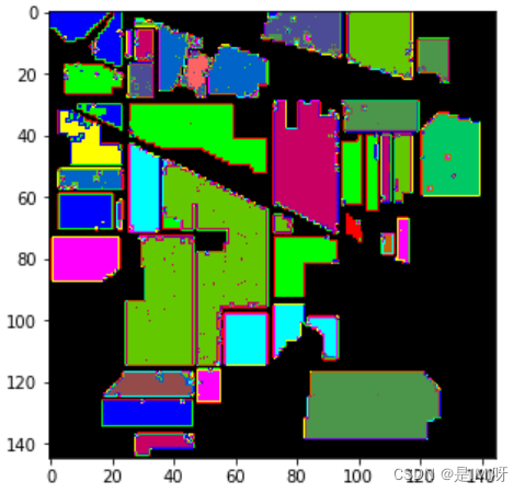
predict_image = spectral.imshow(classes = outputs.astype(int),figsize =(5,5))        

classification map：

问题思考：
1、每次分类结果不相同？
启用dropout后（默认开启了model.train()），会进行随机采样，可能会导致网络在测试时分类结果不一样，准确率可能会受到影响。加入model.eval()可以固定住dropout。

2、如何改进提高准确率？
引入注意力机制，网络会给贡献大的点分配更大的权重，使网络在分类时准确率有提升。