[人工智能]HBU-NNDL 实验四 线性分类

第3章 线性分类

线性回归和线性分类之间有着很大的联系，从某种意义上来说，线性分类就是线性回归函数使用激活函数的结果。同时也可以看成是线性回归降维的结果。对于一个线性回归函数，我们可以通过添加全局函数的形式来将其转换为线性分类函数，

????????????????????????????????????????????????????????????????????????????

3.1 基于Logistic回归的二分类任务

Logistic回归，是一种广义的线性回归分析模型，属于机器学习中的监督学习。其推导过程与计算方式类似于回归的过程，但实际上主要是用来解决二分类问题（也可以解决多分类问题）。通过给定的n组数据（训练集）来训练模型，并在训练结束后对给定的一组或多组数据（测试集）进行分类。其中每一组数据都是由p 个指标构成。

在本节中，我们实现一个Logistic回归模型，并对一个简单的数据集进行二分类实验。

3.1.1 数据集构建

我们首先构建一个简单的分类任务，并构建训练集、验证集和测试集。
本任务的数据来自带噪音的两个弯月形状函数，每个弯月对一个类别。我们采集1000条样本，每个样本包含2个特征。

数据集的构建函数make_moons的代码实现如下：

import math
import copy
import torch


def make_moons(n_samples=1000, shuffle=True, noise=None):
    """
    生成带噪音的弯月形状数据
    输入：
        - n_samples：数据量大小，数据类型为int
        - shuffle：是否打乱数据，数据类型为bool
        - noise：以多大的程度增加噪声，数据类型为None或float，noise为None时表示不增加噪声
    输出：
        - X：特征数据，shape=[n_samples,2]
        - y：标签数据, shape=[n_samples]
    """
    n_samples_out = n_samples // 2
    n_samples_in = n_samples - n_samples_out

    # 采集第1类数据，特征为(x,y)
    # 使用'torch.linspace'在0到pi上均匀取n_samples_out个值
    # 使用'torch.cos'计算上述取值的余弦值作为特征1，使用'torch.sin'计算上述取值的正弦值作为特征2
    outer_circ_x = torch.cos(torch.linspace(0, math.pi, n_samples_out))
    outer_circ_y = torch.sin(torch.linspace(0, math.pi, n_samples_out))

    inner_circ_x = 1 - torch.cos(torch.linspace(0, math.pi, n_samples_in))
    inner_circ_y = 0.5 - torch.sin(torch.linspace(0, math.pi, n_samples_in))

    print('outer_circ_x.shape:', outer_circ_x.shape, 'outer_circ_y.shape:', outer_circ_y.shape)
    print('inner_circ_x.shape:', inner_circ_x.shape, 'inner_circ_y.shape:', inner_circ_y.shape)

    # 使用'torch.concat'将两类数据的特征1和特征2分别延维度0拼接在一起，得到全部特征1和特征2
    # 使用'torch.stack'将两类特征延维度1堆叠在一起
    X = torch.stack(
        [torch.cat([outer_circ_x, inner_circ_x]),
         torch.cat([outer_circ_y, inner_circ_y])],
        dim=1
    )

    print('after concat shape:', torch.cat([outer_circ_x, inner_circ_x]).shape)
    print('X shape:', X.shape)

    # 使用'torch. zeros'将第一类数据的标签全部设置为0
    # 使用'torch. ones'将第一类数据的标签全部设置为1
    y = torch.cat(
        [torch.zeros(size=[n_samples_out]), torch.ones(size=[n_samples_in])]
    )

    print('y shape:', y.shape)

    # 如果shuffle为True，将所有数据打乱
    if shuffle:
        # 使用'torch.randperm'生成一个数值在0到X.shape[0]，随机排列的一维Tensor做索引值，用于打乱数据
        idx = torch.randperm(X.shape[0])
        X = X[idx]
        y = y[idx]

    # 如果noise不为None，则给特征值加入噪声
    if noise is not None:
        # 使用'torch.normal'生成符合正态分布的随机Tensor作为噪声，并加到原始特征上
        X += torch.normal(mean=0.0, std=noise, size=X.shape)

    return X, y

# 采样1000个样本
n_samples = 1000
X, y = make_moons(n_samples=n_samples, shuffle=True, noise=0.5)
# 可视化生产的数据集，不同颜色代表不同类别
import matplotlib.pyplot as plt

plt.figure(figsize=(5,5))
plt.scatter(x=X[:, 0].tolist(), y=X[:, 1].tolist(), marker='*', c=y.tolist())
plt.xlim(-3,4)
plt.ylim(-3,4)
plt.savefig('linear-dataset-vis.pdf')
plt.show()

outer_circ_x.shape: torch.Size([500]) outer_circ_y.shape: torch.Size([500])
inner_circ_x.shape: torch.Size([500]) inner_circ_y.shape: torch.Size([500])
after concat shape: torch.Size([1000])
X shape: torch.Size([1000, 2])
y shape: torch.Size([1000])

将1000条样本数据拆分成训练集、验证集和测试集，其中训练集640条、验证集160条、测试集200条。代码实现如下：

num_train = 640     #训练集
num_dev = 160       #验证集
num_test = 200      #测试集

X_train, y_train = X[:num_train], y[:num_train]
X_dev, y_dev = X[num_train:num_train + num_dev], y[num_train:num_train + num_dev]
X_test, y_test = X[num_train + num_dev:], y[num_train + num_dev:]

y_train = y_train.reshape([-1,1])
y_dev = y_dev.reshape([-1,1])
y_test = y_test.reshape([-1,1])

# 打印X_train和y_train的维度
print("X_train shape: ", X_train.shape, "y_train shape: ", y_train.shape)

# 打印一下前5个数据的标签
print (y_train[:5])

X_train shape: ?torch.Size([640, 2]) y_train shape: ?torch.Size([640, 1])
tensor([[1.],
? ? ? ? [0.],
? ? ? ? [1.],
? ? ? ? [0.],
? ? ? ? [1.]])

3.1.2 模型构建

Logistic函数

Logistic函数的代码实现如下：

def logistic(x):
    return 1/(1+torch.exp(-x))

# 在[-10,10]的范围内生成一系列的输入值，用于绘制函数曲线
x = torch.linspace(-10, 10, 10000)
plt.figure()
plt.plot(x, logistic(x),label="Logistic Function")
# 设置坐标轴
ax = plt.gca()
# 取消右侧和上侧坐标轴
ax.spines['top'].set_color('none')
ax.spines['right'].set_color('none')
# 设置默认的x轴和y轴方向
ax.xaxis.set_ticks_position('bottom')
ax.yaxis.set_ticks_position('left')
# 设置坐标原点为(0,0)
ax.spines['left'].set_position(('data',0))
ax.spines['bottom'].set_position(('data',0))
# 添加图例
plt.legend()
plt.savefig('linear-logistic.pdf')
plt.show()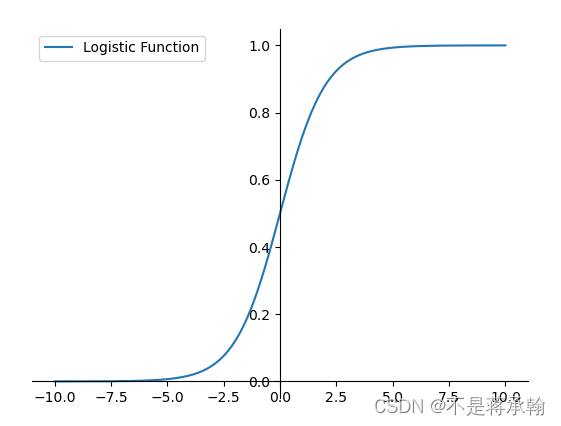

这个logistic函数也就是我们常说的sigmoid函数?

?

问题1：Logistic回归在不同的书籍中，有许多其他的称呼，具体有哪些？你认为哪个称呼最好？

logistic regression 翻译成中文的译本却是有几个，逻辑回归（大家常说的），对数几率回归（周志华机器学习书籍），逻辑斯谛回归（Understanding Machine Learning：From Theory to Algorithms中译本）。
从单词（词根）的角度：

logistic adj.逻辑的；n.数理（符号）逻辑，逻辑斯蒂
   ↓
logic 译为 n.逻辑 adj.逻辑的，这词是个舶来品，是音译
大家常说的的【逻辑回归算法】中的【逻辑】不是中文常说的【逻辑思维】这种逻辑。或译成：逻辑斯蒂回归。以避免误导性。
logistic指的是 logistic函数

-------------------------------------------------------------

regression =     re     +        gress                +   sion
                  ↓                 ↓                        ↓
           回/向后/相反 | to go/walk行走，来自拉丁语    | 名词后缀
=>翻译：向后走

?根据上述推导过程，我认为最准确的翻译应该是：对数几率回归

问题2：什么是激活函数？为什么要用激活函数？常见激活函数有哪些？

如“激活”一词所示，激活函数的作用在于决定如何来激活输入信号的总和。

关于激活函数的作用，借用斋藤老师的鱼书上的一段话

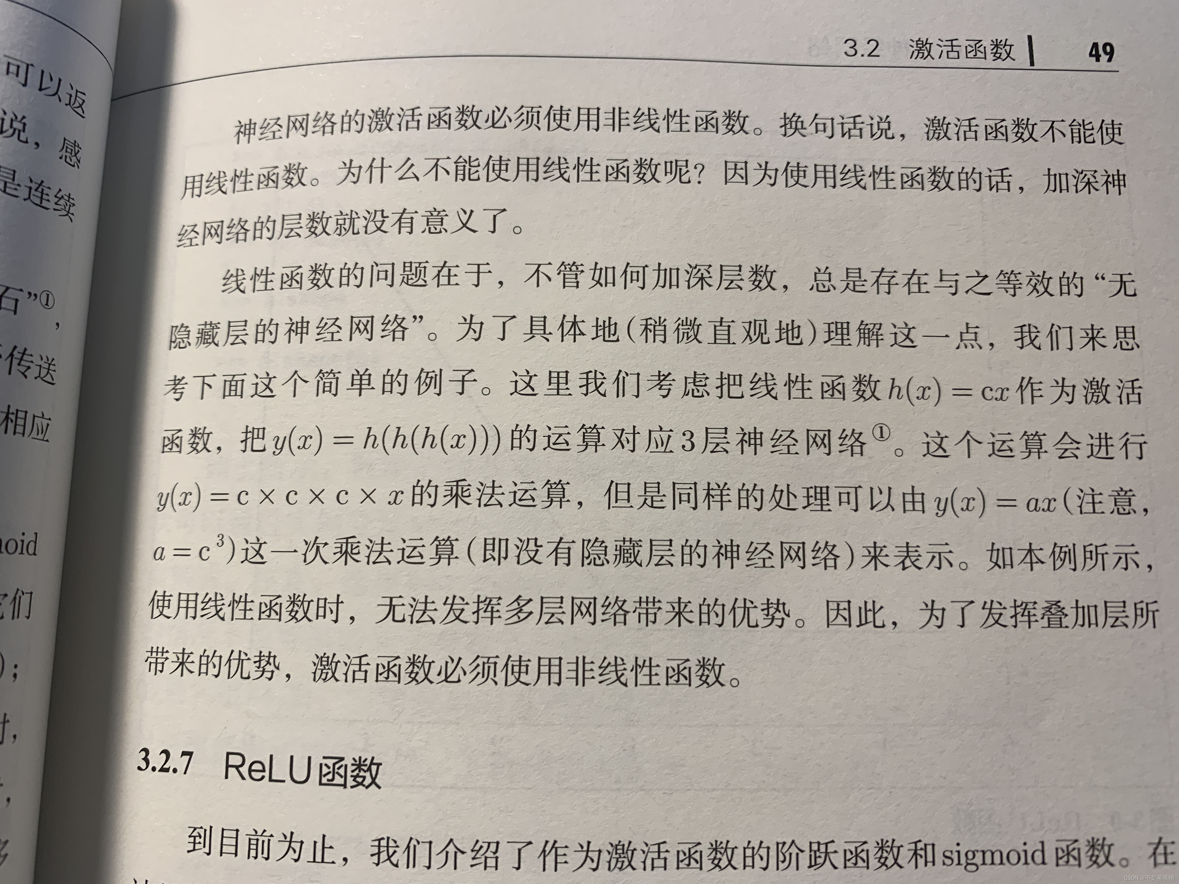
?上述非线性函数的作用就是激活函数的作用。

常见的激活函数有：阶跃函数、sigmoid函数（logistic函数）、softmax函数、ReLU函数、tanh函数。

Logistic回归算子

Logistic回归模型其实就是线性层与Logistic函数的组合，通常会将 Logistic回归模型中的权重和偏置初始化为0，同时，为了提高预测样本的效率，我们将N个样本归为一组进行成批地预测。

import op

class model_LR(op.Op):
    def __init__(self, input_dim):
        super(model_LR, self).__init__()
        self.params = {}
        # 将线性层的权重参数全部初始化为0
        self.params['w'] = torch.zeros(size=[input_dim, 1])
        # self.params['w'] = paddle.normal(mean=0, std=0.01, shape=[input_dim, 1])
        # 将线性层的偏置参数初始化为0
        self.params['b'] = torch.zeros(size=[1])

    def __call__(self, inputs):
        return self.forward(inputs)

    def forward(self, inputs):
        """
        输入：
            - inputs: shape=[N,D], N是样本数量，D为特征维度
        输出：
            - outputs：预测标签为1的概率，shape=[N,1]
        """
        # 线性计算
        score = torch.matmul(inputs, self.params['w']) + self.params['b']
        # Logistic 函数
        outputs = logistic(score)
        return outputs

模型测试

# 固定随机种子，保持每次运行结果一致
torch.manual_seed(0)
# 随机生成3条长度为4的数据
inputs = torch.randn(size=[3,4])
print('Input is:', inputs)
# 实例化模型
model = model_LR(4)
outputs = model(inputs)
print('Output is:', outputs)

Input is: tensor([[ 1.5410, -0.2934, -2.1788, ?0.5684],
? ? ? ? [-1.0845, -1.3986, ?0.4033, ?0.8380],
? ? ? ? [-0.7193, -0.4033, -0.5966, ?0.1820]])
Output is: tensor([[0.5000],
? ? ? ? [0.5000],
? ? ? ? [0.5000]])

3.1.3 损失函数

二分类任务的交叉熵损失函数的代码实现如下：

class BinaryCrossEntropyLoss(op.Op):
    def __init__(self):
        self.predicts = None
        self.labels = None
        self.num = None

    def __call__(self, predicts, labels):
        return self.forward(predicts, labels)

    def forward(self, predicts, labels):
        """
        输入：
            - predicts：预测值，shape=[N, 1]，N为样本数量
            - labels：真实标签，shape=[N, 1]
        输出：
            - 损失值：shape=[1]
        """
        self.predicts = predicts
        self.labels = labels
        self.num = self.predicts.shape[0]
        loss = -1. / self.num * (torch.matmul(self.labels.t(), torch.log(self.predicts)) + torch.matmul((1-self.labels.t()), torch.log(1-self.predicts)))
        loss = torch.squeeze(loss, dim=1)
        return loss

测试交叉熵损失函数

# 生成一组长度为3，值为1的标签数据
labels = torch.ones(size=[3,1])
# 计算风险函数
bce_loss = BinaryCrossEntropyLoss()
print('交叉熵损失为：',bce_loss(outputs, labels))

交叉熵损失为： tensor([0.6931])

3.1.4 模型优化

不同于线性回归中直接使用最小二乘法即可进行模型参数的求解，Logistic回归需要使用优化算法对模型参数进行有限次地迭代来获取更优的模型，从而尽可能地降低风险函数的值。
在机器学习任务中，最简单、常用的优化算法是梯度下降法。

使用梯度下降法进行模型优化，首先需要初始化参数W和?b，然后不断地计算它们的梯度，并沿梯度的反方向更新参数。

3.1.4.1 梯度计算

在Logistic回归中，风险函数R(w,b)关于参数w和b的偏导数为：

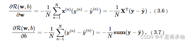
?通常将偏导数的计算过程定义在Logistic回归算子的backward函数中，代码实现如下:

    def backward(self, labels):
        """
        输入：
            - labels：真实标签，shape=[N, 1]
        """
        N = labels.shape[0]
        # 计算偏导数
        self.grads['w'] = -1 / N * torch.matmul(self.X.t(), (labels - self.outputs))
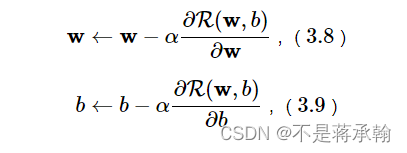
        self.grads['b'] = -1 / N * torch.sum(labels - self.outputs)

3.1.4.2 参数更新

在计算参数的梯度之后，我们按照下面公式更新参数：

?

首先定义一个优化器基类Optimizer，方便后续所有的优化器调用。在这个基类中，需要初始化优化器的初始学习率init_lr，以及指定优化器需要优化的参数。代码实现如下：

class Optimizer(object):
    def __init__(self, init_lr, model):
        """
        优化器类初始化
        """
        # 初始化学习率，用于参数更新的计算
        self.init_lr = init_lr
        # 指定优化器需要优化的模型
        self.model = model

    @abstractmethod
    def step(self):
        """
        定义每次迭代如何更新参数
        """
        pass

然后实现一个梯度下降法的优化器函数SimpleBatchGD来执行参数更新过程。其中step函数从模型的grads属性取出参数的梯度并更新。代码实现如下：

class SimpleBatchGD(Optimizer):
    def __init__(self, init_lr, model):
        super(SimpleBatchGD, self).__init__(init_lr=init_lr, model=model)

    def step(self):
        # 参数更新
        # 遍历所有参数，按照公式(3.8)和(3.9)更新参数
        if isinstance(self.model.params, dict):
            for key in self.model.params.keys():
                self.model.params[key] = self.model.params[key] - self.init_lr * self.model.grads[key]

3.1.5 评价指标

在分类任务中，通常使用准确率（Accuracy）作为评价指标。如果模型预测的类别与真实类别一致，则说明模型预测正确。准确率即正确预测的数量与总的预测数量的比值：

?

def accuracy(preds, labels):
    """
    输入：
        - preds：预测值，二分类时，shape=[N, 1]，N为样本数量，多分类时，shape=[N, C]，C为类别数量
        - labels：真实标签，shape=[N, 1]
    输出：
        - 准确率：shape=[1]
    """
    # 判断是二分类任务还是多分类任务，preds.shape[1]=1时为二分类任务，preds.shape[1]>1时为多分类任务
    if preds.shape[1] == 1:
        data_float = torch.randn(preds.shape[0], preds.shape[1])
        # 二分类时，判断每个概率值是否大于0.5，当大于0.5时，类别为1，否则类别为0
        # 使用'torch.cast'将preds的数据类型转换为float32类型
        preds = (preds>=0.5).type(torch.float32)
    else:
        # 多分类时，使用'torch.argmax'计算最大元素索引作为类别
        data_float = torch.randn(preds.shape[0], preds.shape[1])
        preds = torch.argmax(preds,dim=1, dtype=torch.int32)
    return torch.mean(torch.eq(preds, labels).type(torch.float32))

测试一下

# 假设模型的预测值为[[0.],[1.],[1.],[0.]]，真实类别为[[1.],[1.],[0.],[0.]]，计算准确率
preds = torch.tensor([[0.],[1.],[1.],[0.]])
labels = torch.tensor([[1.],[1.],[0.],[0.]])
print("accuracy is:", accuracy(preds, labels))

accuracy is: tensor(0.5000)

3.1.6 完善Runner类

基于RunnerV1，本章的RunnerV2类在训练过程中使用梯度下降法进行网络优化，模型训练过程中计算在训练集和验证集上的损失及评估指标并打印，训练过程中保存最优模型。代码实现如下：

# 用RunnerV2类封装整个训练过程
class RunnerV2(object):
    def __init__(self, model, optimizer, metric, loss_fn):
        self.model = model
        self.optimizer = optimizer
        self.loss_fn = loss_fn
        self.metric = metric
        # 记录训练过程中的评价指标变化情况
        self.train_scores = []
        self.dev_scores = []
        # 记录训练过程中的损失函数变化情况
        self.train_loss = []
        self.dev_loss = []

    def train(self, train_set, dev_set, **kwargs):
        # 传入训练轮数，如果没有传入值则默认为0
        num_epochs = kwargs.get("num_epochs", 0)
        # 传入log打印频率，如果没有传入值则默认为100
        log_epochs = kwargs.get("log_epochs", 100)
        # 传入模型保存路径，如果没有传入值则默认为"best_model.pdparams"
        save_path = kwargs.get("save_path", "best_model.pdparams")
        # 梯度打印函数，如果没有传入则默认为"None"
        print_grads = kwargs.get("print_grads", None)
        # 记录全局最优指标
        best_score = 0
        # 进行num_epochs轮训练
        for epoch in range(num_epochs):
            X, y = train_set
            # 获取模型预测
            logits = self.model(X)
            # 计算交叉熵损失
            trn_loss = self.loss_fn(logits, y).item()
            self.train_loss.append(trn_loss)
            # 计算评价指标
            trn_score = self.metric(logits, y).item()
            self.train_scores.append(trn_score)
            # 计算参数梯度
            self.model.backward(y)
            if print_grads is not None:
                # 打印每一层的梯度
                print_grads(self.model)
            # 更新模型参数
            self.optimizer.step()
            dev_score, dev_loss = self.evaluate(dev_set)
            # 如果当前指标为最优指标，保存该模型
            if dev_score > best_score:
                self.save_model(save_path)
                print(f"best accuracy performence has been updated: {best_score:.5f} --> {dev_score:.5f}")
                best_score = dev_score
            if epoch % log_epochs == 0:
                print(f"[Train] epoch: {epoch}, loss: {trn_loss}, score: {trn_score}")
                print(f"[Dev] epoch: {epoch}, loss: {dev_loss}, score: {dev_score}")

    def evaluate(self, data_set):
        X, y = data_set
        # 计算模型输出
        logits = self.model(X)
        # 计算损失函数
        loss = self.loss_fn(logits, y).item()
        self.dev_loss.append(loss)
        # 计算评价指标
        score = self.metric(logits, y).item()
        self.dev_scores.append(score)
        return score, loss

    def predict(self, X):
        return self.model(X)

    def save_model(self, save_path):
        torch.save(self.model.params, save_path)

    def load_model(self, model_path):
        self.model.params = torch.load(model_path)

3.1.7 模型训练

下面进行Logistic回归模型的训练，使用交叉熵损失函数和梯度下降法进行优化。
使用训练集和验证集进行模型训练，共训练 500个epoch，每隔50个epoch打印出训练集上的指标。
代码实现如下：

# 固定随机种子，保持每次运行结果一致
torch.manual_seed(102)

# 特征维度
input_dim = 2
# 学习率
lr = 0.1

# 实例化模型
model = model_LR(input_dim=input_dim)
# 指定优化器
optimizer = SimpleBatchGD(init_lr=lr, model=model)
# 指定损失函数
loss_fn = BinaryCrossEntropyLoss()
# 指定评价方式
metric = accuracy

# 实例化RunnerV2类，并传入训练配置
runner = RunnerV2(model, optimizer, metric, loss_fn)

runner.train([X_train, y_train], [X_dev, y_dev], num_epochs=500, log_epochs=50, save_path="best_model.pdparams")

best accuracy performence has been updated: 0.00000 --> 0.77500
[Train] epoch: 0, loss: 0.6931460499763489, score: 0.5218750238418579
[Dev] epoch: 0, loss: 0.6839450001716614, score: 0.7749999761581421
best accuracy performence has been updated: 0.77500 --> 0.78125
[Train] epoch: 50, loss: 0.4823344349861145, score: 0.7953125238418579
[Dev] epoch: 50, loss: 0.5100909471511841, score: 0.768750011920929
[Train] epoch: 100, loss: 0.43836650252342224, score: 0.792187511920929
[Dev] epoch: 100, loss: 0.4771150052547455, score: 0.7562500238418579
[Train] epoch: 150, loss: 0.420661062002182, score: 0.796875
[Dev] epoch: 150, loss: 0.4678696095943451, score: 0.762499988079071
[Train] epoch: 200, loss: 0.41160938143730164, score: 0.7953125238418579
[Dev] epoch: 200, loss: 0.46574288606643677, score: 0.78125
[Train] epoch: 250, loss: 0.4063630700111389, score: 0.796875
[Dev] epoch: 250, loss: 0.46621155738830566, score: 0.78125
[Train] epoch: 300, loss: 0.40308570861816406, score: 0.796875
[Dev] epoch: 300, loss: 0.46767398715019226, score: 0.78125
best accuracy performence has been updated: 0.78125 --> 0.78750
[Train] epoch: 350, loss: 0.4009374678134918, score: 0.800000011920929
[Dev] epoch: 350, loss: 0.46947580575942993, score: 0.7875000238418579
[Train] epoch: 400, loss: 0.3994828760623932, score: 0.800000011920929
[Dev] epoch: 400, loss: 0.4713282585144043, score: 0.7875000238418579
[Train] epoch: 450, loss: 0.39847469329833984, score: 0.8031250238418579
[Dev] epoch: 450, loss: 0.47310104966163635, score: 0.7875000238418579
best accuracy performence has been updated: 0.78750 --> 0.79375

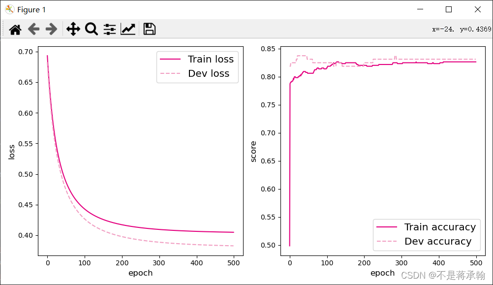
可视化观察训练集与验证集的准确率和损失的变化情况。

# 可视化观察训练集与验证集的指标变化情况
def plot(runner,fig_name):
    plt.figure(figsize=(10,5))
    plt.subplot(1,2,1)
    epochs = [i for i in range(len(runner.train_scores))]
    # 绘制训练损失变化曲线
    plt.plot(epochs, runner.train_loss, color='#e4007f', label="Train loss")
    # 绘制评价损失变化曲线
    plt.plot(epochs, runner.dev_loss, color='#f19ec2', linestyle='--', label="Dev loss")
    # 绘制坐标轴和图例
    plt.ylabel("loss", fontsize='large')
    plt.xlabel("epoch", fontsize='large')
    plt.legend(loc='upper right', fontsize='x-large')
    plt.subplot(1,2,2)
    # 绘制训练准确率变化曲线
    plt.plot(epochs, runner.train_scores, color='#e4007f', label="Train accuracy")
    # 绘制评价准确率变化曲线
    plt.plot(epochs, runner.dev_scores, color='#f19ec2', linestyle='--', label="Dev accuracy")
    # 绘制坐标轴和图例
    plt.ylabel("score", fontsize='large')
    plt.xlabel("epoch", fontsize='large')
    plt.legend(loc='lower right', fontsize='x-large')
    plt.tight_layout()
    plt.savefig(fig_name)
    plt.show()

plot(runner,fig_name='linear-acc.pdf')

3.1.8 模型评价

使用测试集对训练完成后的最终模型进行评价，观察模型在测试集上的准确率和loss数据。代码实现如下：

score, loss = runner.evaluate([X_test, y_test])
print("[Test] score/loss: {:.4f}/{:.4f}".format(score, loss))

[Test] score/loss: 0.7650/0.4378

调整学习率为0.5后：

[Test] score/loss: 0.8250/0.4047

发现score上升，loss下降，

调整学习率为0.01后：

[Test] score/loss: 0.7100/0.5410

从自己和其他人一般的经验来看，学习率可以设置为3、1、0.5、0.1、0.05、0.01、0.005，0.005、0.0001、0.00001具体需结合实际情况对比判断，小的学习率收敛慢，还会将loss值升高。

调整epoch为5000后：

[Test] score/loss: 0.8050/0.4063

发现score上升，loss下降

调整epoch为10000后：

[Test] score/loss: 0.7850/0.4704

发现score下降，loss上升

此时模型应该发生了过拟合导致准确率下降。

可视化观察拟合的决策边界 。

def decision_boundary(w, b, x1):
    w1, w2 = w
    x2 = (- w1 * x1 - b) / w2
    return x2

plt.figure(figsize=(5,5))
# 绘制原始数据
plt.scatter(X[:, 0].tolist(), X[:, 1].tolist(), marker='*', c=y.tolist())

w = model.params['w']
b = model.params['b']
x1 = torch.linspace(-2, 3, 1000)
x2 = decision_boundary(w, b, x1)
# 绘制决策边界
plt.plot(x1.tolist(), x2.tolist(), color="red")
plt.show()

3.2 基于Softmax回归的多分类任务

Logistic回归可以有效地解决二分类问题，但在分类任务中，还有一类多分类问题，即类别数C大于2 的分类问题。Softmax回归就是Logistic回归在多分类问题上的推广。

使用Softmax回归模型对一个简单的数据集进行多分类实验。

3.2.1 数据集构建

我们首先构建一个简单的多分类任务，并构建训练集、验证集和测试集。
本任务的数据来自3个不同的簇，每个簇对一个类别。我们采集1000条样本，每个样本包含2个特征。

数据集的构建函数make_multi的代码实现如下：

def make_multiclass_classification(n_samples=100, n_features=2, n_classes=3, shuffle=True, noise=0.1):
    """
    生成带噪音的多类别数据
    输入：
        - n_samples：数据量大小，数据类型为int
        - n_features：特征数量，数据类型为int
        - shuffle：是否打乱数据，数据类型为bool
        - noise：以多大的程度增加噪声，数据类型为None或float，noise为None时表示不增加噪声
    输出：
        - X：特征数据，shape=[n_samples,2]
        - y：标签数据, shape=[n_samples,1]
    """
    # 计算每个类别的样本数量
    n_samples_per_class = [int(n_samples / n_classes) for k in range(n_classes)]
    for i in range(n_samples - sum(n_samples_per_class)):
        n_samples_per_class[i % n_classes] += 1
    # 将特征和标签初始化为0
    X = torch.zeros([n_samples, n_features])
    y = torch.zeros([n_samples], dtype=torch.int32)
    # 随机生成3个簇中心作为类别中心
    centroids = torch.randperm(2 ** n_features)[:n_classes]
    centroids_bin = np.unpackbits(centroids.numpy().astype('uint8')).reshape((-1, 8))[:, -n_features:]
    centroids = torch.tensor(centroids_bin, dtype=torch.float32)
    # 控制簇中心的分离程度
    centroids = 1.5 * centroids - 1
    # 随机生成特征值
    X[:, :n_features] = torch.randn(size=[n_samples, n_features])

    stop = 0
    # 将每个类的特征值控制在簇中心附近
    for k, centroid in enumerate(centroids):
        start, stop = stop, stop + n_samples_per_class[k]
        # 指定标签值
        y[start:stop] = k % n_classes
        X_k = X[start:stop, :n_features]
        # 控制每个类别特征值的分散程度
        A = 2 * torch.rand(size=[n_features, n_features]) - 1
        X_k[...] = torch.matmul(X_k, A)
        X_k += centroid
        X[start:stop, :n_features] = X_k

    # 如果noise不为None，则给特征加入噪声
    if noise > 0.0:
        # 生成noise掩膜，用来指定给那些样本加入噪声
        noise_mask = torch.rand([n_samples]) < noise
        for i in range(len(noise_mask)):
            if noise_mask[i]:
                # 给加噪声的样本随机赋标签值
                y[i] = torch.randint(n_classes, size=[1]).type(torch.int32)
    # 如果shuffle为True，将所有数据打乱
    if shuffle:
        idx = torch.randperm(X.shape[0])
        X = X[idx]
        y = y[idx]

    return X, y

随机采集1000个样本，并进行可视化。

# 固定随机种子，保持每次运行结果一致
torch.manual_seed(102)
# 采样1000个样本
n_samples = 1000
X, y = make_multiclass_classification(n_samples=n_samples, n_features=2, n_classes=3, noise=0.2)

import matplotlib.pyplot as plt

# 可视化生产的数据集，不同颜色代表不同类别
plt.figure(figsize=(5,5))
plt.scatter(x=X[:, 0].tolist(), y=X[:, 1].tolist(), marker='*', c=y.tolist())
plt.savefig('linear-dataset-vis2.pdf')
plt.show()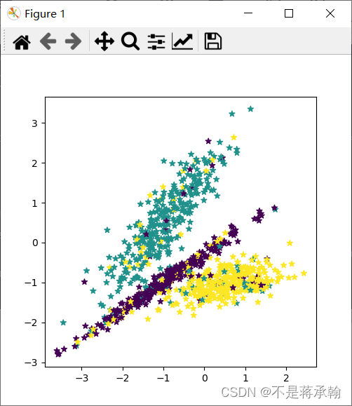

将实验数据拆分成训练集、验证集和测试集。其中训练集640条、验证集160条、测试集200条。

num_train = 640
num_dev = 160
num_test = 200

X_train, y_train = X[:num_train], y[:num_train]
X_dev, y_dev = X[num_train:num_train + num_dev], y[num_train:num_train + num_dev]
X_test, y_test = X[num_train + num_dev:], y[num_train + num_dev:]

# 打印X_train和y_train的维度
print("X_train shape: ", X_train.shape, "y_train shape: ", y_train.shape)

X_train shape: ?torch.Size([640, 2]) y_train shape: ?torch.Size([640])

3.2.2 模型构建

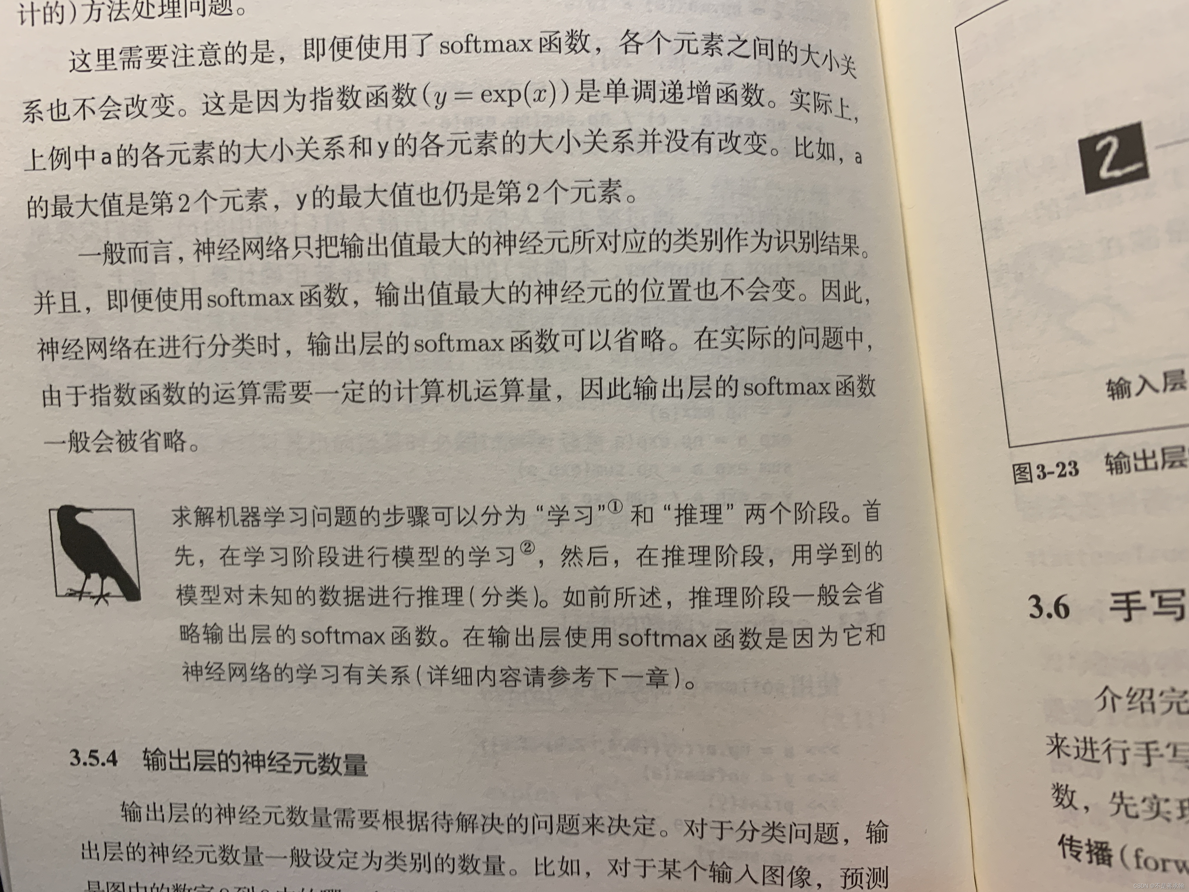
在Softmax回归中，对类别进行预测的方式是预测输入属于每个类别的条件概率。与Logistic 回归不同的是，Softmax回归的输出值个数等于类别数C，而每个类别的概率值则通过Softmax函数进行求解。

3.2.2.1 Softmax函数

首先我们先建立一个如下标准的softmax

?

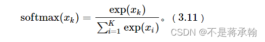# x为tensor
def softmax(X):
    """
    输入：
        - X：shape=[N, C]，N为向量数量，C为向量维度
    """
    x_exp = torch.exp(X)
    partition = torch.sum(x_exp, dim=1, keepdim=True)#N,1
    return x_exp / partition

但是这个softmax不够好，会出错，下面再次借用斋藤老师鱼书上的一些东西：

?

?

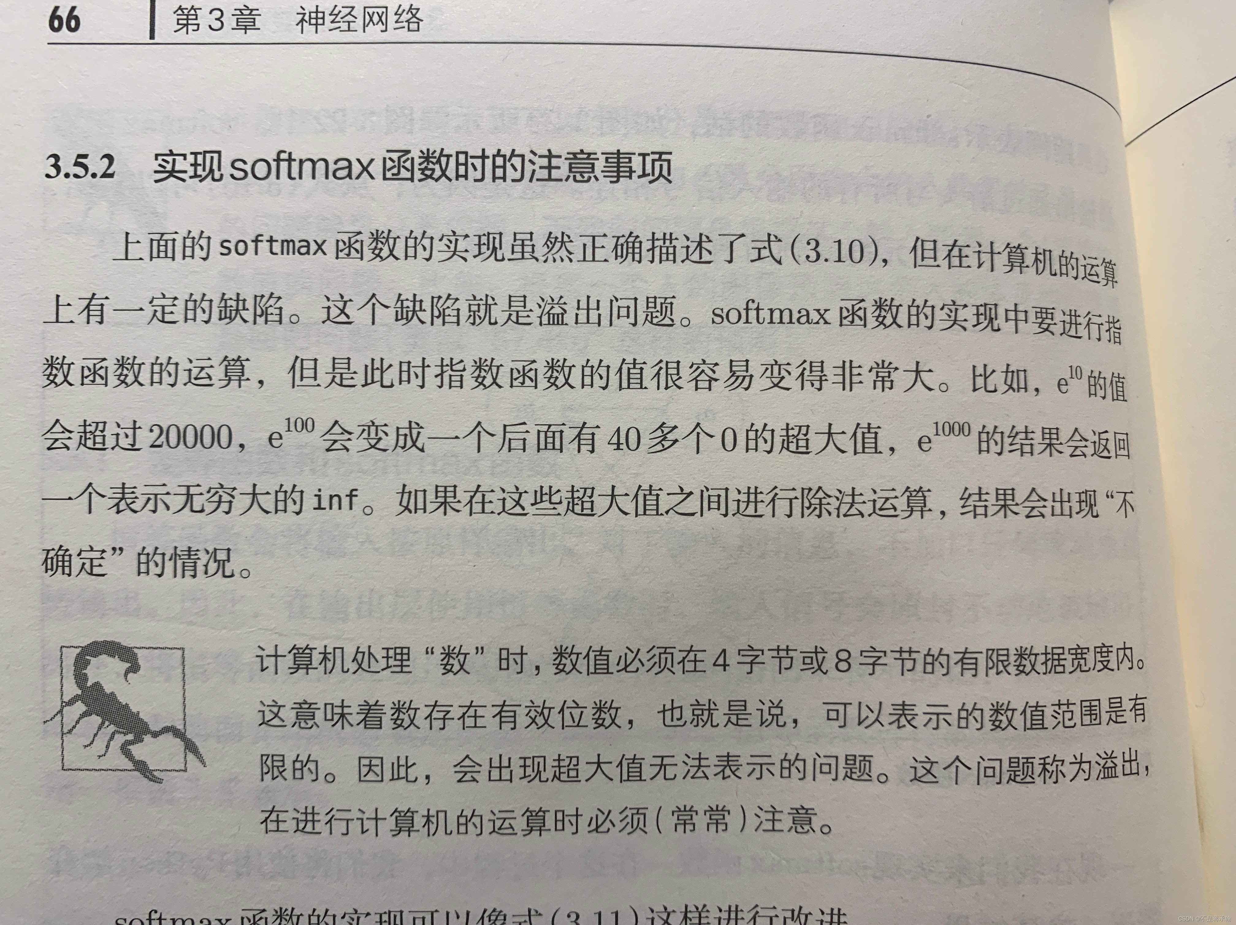
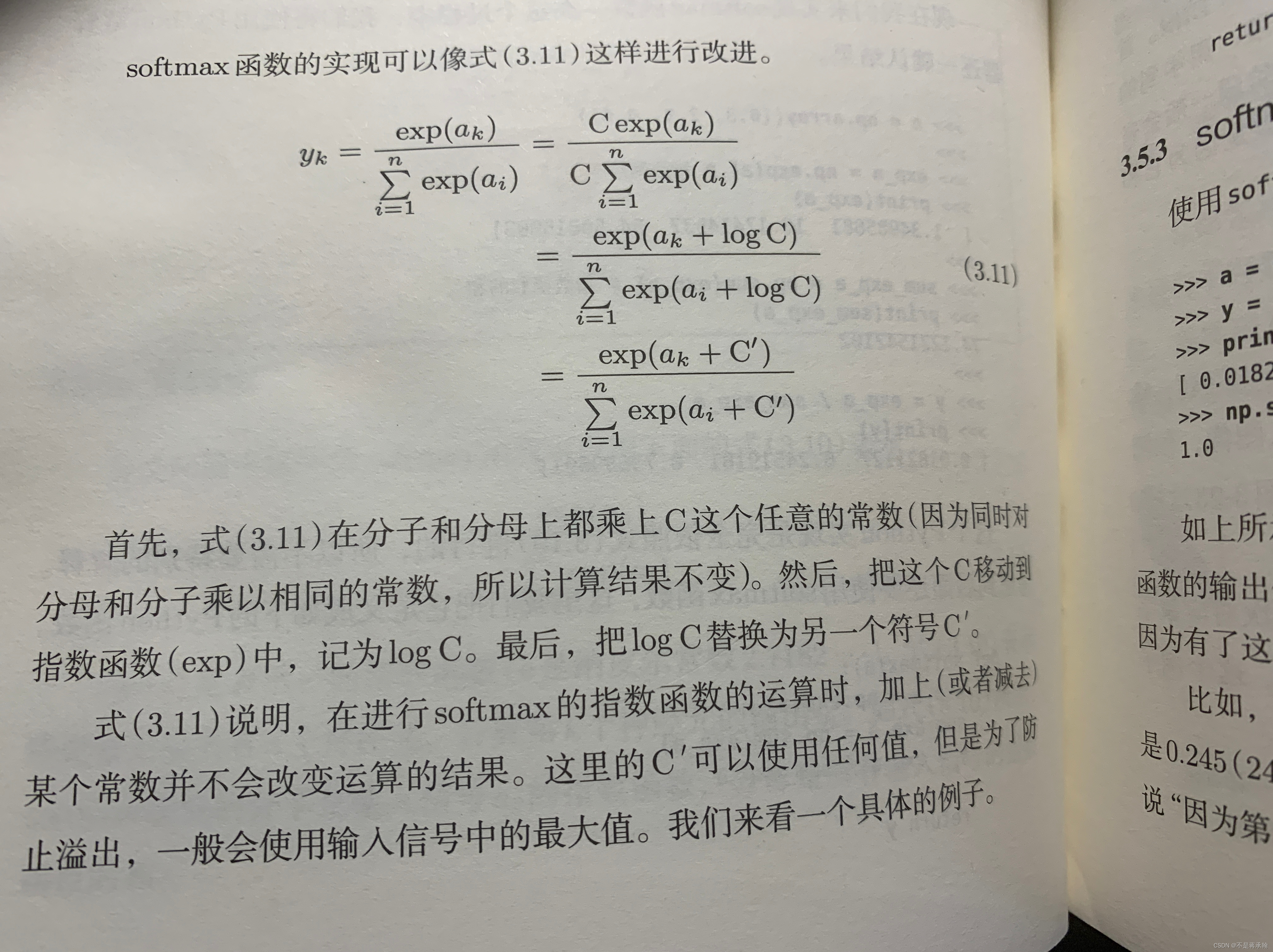
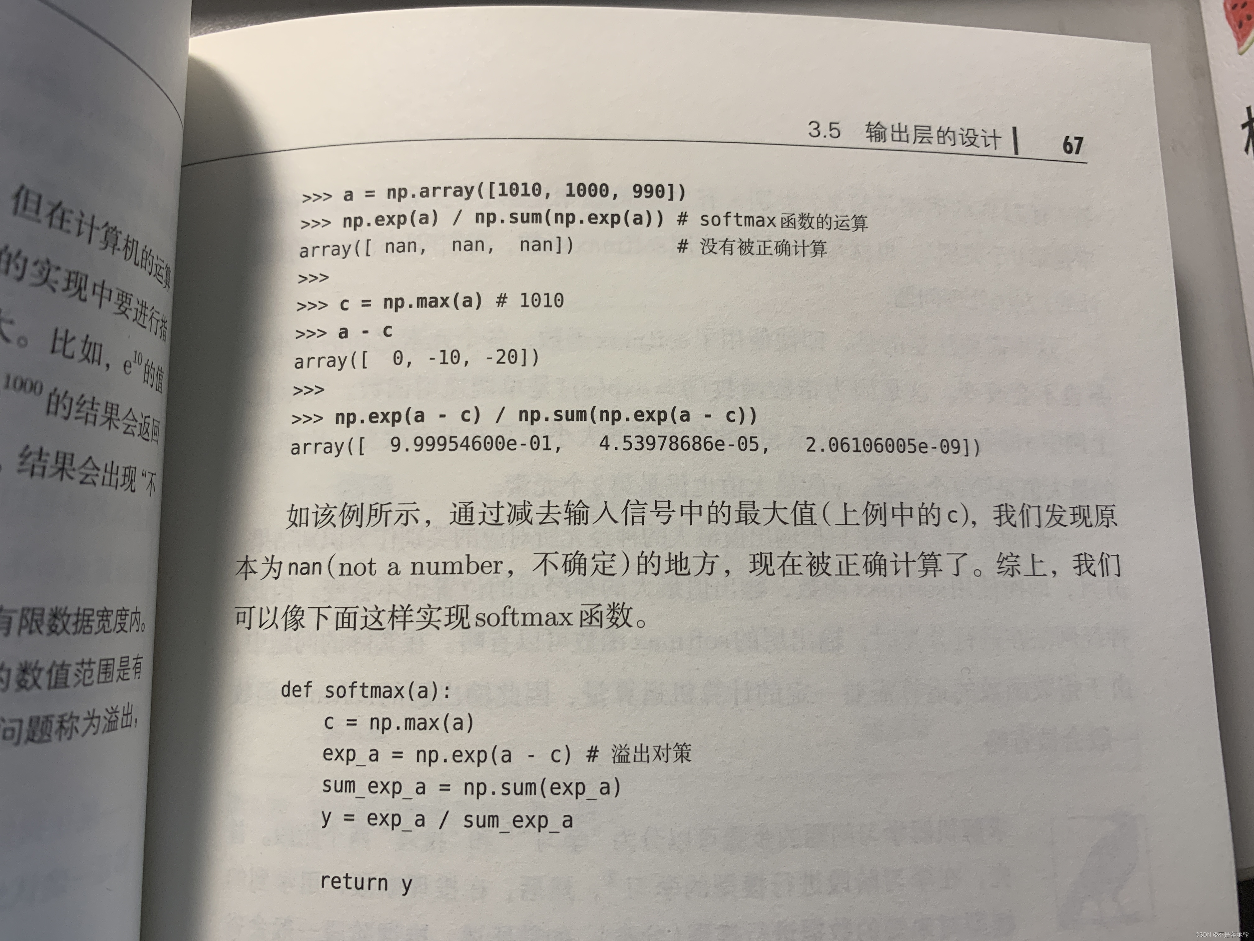
所以我们用pytorch实现改良后的softmax函数?

# x为tensor
def softmax(X):
    """
    输入：
        - X：shape=[N, C]，N为向量数量，C为向量维度
    """
    x_max = torch.max(X, dim=1, keepdim=True)[0]#N,1
    x_exp = torch.exp(X - x_max)
    partition = torch.sum(x_exp, dim=1, keepdim=True)#N,1
    return x_exp / partition

?x_max的类型不是tensor，是由最大值和最大值下标组成的，我们只要最大值tensor，所以加个[0]

softmax函数其实是从hardmax演变而来的，hardmax函数其实是我们生活中很常见的一种函数，表达式是：

表达的意思很清楚，从写，y和x中取较大的那个值，为了方便后续比较，我们将hardmax的形式换一下：

此时，函数本质功能没变，我们只是对定义域做了一个限制，即：

?其图形如下：

?很显然这个函数在 x = 1 处是连续不可导的，可导能帮我们做很多事，那我们有没有办法对他变形，找到一个连续可导的近似函数？

此时就有了softmax函数：

我们先来看一下这个代数表达式的数学特性。指数函数有一个特点，就是变化率非常快。当x>y时，通过指数的放大作用，会使得二者差距进一步变大，即：

所以有：

所以g(x，y)表达式有：

因此根据上面的推导过程，g(x，y)约等于x，y中较大的值，即：

所以我们得出一个结论，g(x，y)是max{x，y}的近似函数，两个函数有相似的数学特性。我们再来看一下softmax函数的图像：

?

很显然这是一个连续且处处可导的函数，这是一个非常重要的特性，g(x，y)即具有与max{x，y}的相似性，又避免了max{x，y}函数不可导的缺点。

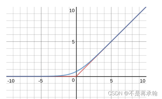
我们把两张图叠加到一起来看看，红色的折线是hardmax函数，他有一个尖尖的棱角，看起来很"hard"。蓝色的弧线看起来就平滑的多，不那么"hard"，这就是softmax函数了。这就时softmax函数名称的由来。

从图上可以看出，当x，y的差别越大时，softmax和hardmax函数吻合度越高。

?

?思考题：Logistic函数是激活函数。Softmax函数是激活函数么？谈谈你的看法。

咱们继续来看看鱼书

?SoftMax定义了神经网络新型的输出方法，其实这一过程主要是增加神经网络对训练集的拟合程度，将线性（隐层第一步的WX+b）转变成非线性，不改变神经网络的加权输入，从而加大了神经网络的灵活度。

3.2.2.2 Softmax回归算子

我们根据公式

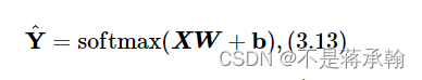实现Softmax回归算子，代码实现如下：

class model_SR(op.Op):
    def __init__(self, input_dim, output_dim):
        super(model_SR, self).__init__()
        self.params = {}
        # 将线性层的权重参数全部初始化为0
        self.params['W'] = torch.zeros(size=[input_dim, output_dim])
        # self.params['W'] = torch.normal(mean=0, std=0.01, shape=[input_dim, output_dim])
        # 将线性层的偏置参数初始化为0
        self.params['b'] = torch.zeros(size=[output_dim])
        self.outputs = None

    def __call__(self, inputs):
        return self.forward(inputs)

    def forward(self, inputs):
        """
        输入：
            - inputs: shape=[N,D], N是样本数量，D是特征维度
        输出：
            - outputs：预测值，shape=[N,C]，C是类别数
        """
        # 线性计算
        score = torch.matmul(inputs, self.params['W']) + self.params['b']
        # Softmax 函数
        self.outputs = softmax(score)
        return self.outputs

# 随机生成1条长度为4的数据
inputs = torch.randn(size=[1,4])
print('Input is:', inputs)
# 实例化模型，这里令输入长度为4，输出类别数为3
model = model_SR(input_dim=4, output_dim=3)
outputs = model(inputs)
print('Output is:', outputs)

Input is: tensor([[-0.6014, -1.0122, -0.3023, -1.2277]])
Output is: tensor([[0.3333, 0.3333, 0.3333]])

3.2.3 损失函数

Softmax回归同样使用交叉熵损失作为损失函数，并使用梯度下降法对参数进行优化。

因此，多类交叉熵损失函数的代码实现如下：

class MultiCrossEntropyLoss(op.Op):
    def __init__(self):
        self.predicts = None
        self.labels = None
        self.num = None

    def __call__(self, predicts, labels):
        return self.forward(predicts, labels)

    def forward(self, predicts, labels):
        """
        输入：
            - predicts：预测值，shape=[N, 1]，N为样本数量
            - labels：真实标签，shape=[N, 1]
        输出：
            - 损失值：shape=[1]
        """
        self.predicts = predicts
        self.labels = labels
        self.num = self.predicts.shape[0]
        loss = 0
        for i in range(0, self.num):
            index = self.labels[i]
            loss -= torch.log(self.predicts[i][index])
        return loss / self.num

# 假设真实标签为第1类
labels = torch.tensor([0])
# 计算风险函数
mce_loss = MultiCrossEntropyLoss()
print(mce_loss(outputs, labels))

tensor(1.0986)

3.2.4 模型优化

使用梯度下降法进行参数学习。

3.2.4.1 梯度计算

计算风险函数R(W,b)关于参数W和b的偏导数。在Softmax回归中，计算方法为：

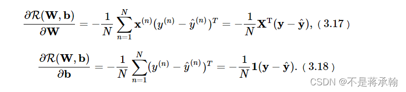
    def backward(self, labels):
        """
        输入：
            - labels：真实标签，shape=[N, 1]，其中N为样本数量
        """
        # 计算偏导数
        N =labels.shape[0]
        labels = torch.nn.functional.one_hot(labels, self.output_dim)
        self.grads['W'] = -1 / N * torch.matmul(self.X.t(), (labels-self.outputs))
        self.grads['b'] = -1 / N * torch.matmul(torch.ones(size=[N]), (labels-self.outputs))

?此函数使用torch.nn.functional.one_hot时会报错：

one_hot is only applicable to index tensor.

原因是创建数据集时

y = torch.zeros([n_samples], dtype=torch.int32)

这样转化过来的tensor，pytorch是不会为其构建索引的,所以要将int32改为int64

3.2.4.2 参数更新

在计算参数的梯度之后，我们使用3.1.4.2中实现的梯度下降法进行参数更新。

from abc import abstractmethod

# 优化器基类
class Optimizer(object):
    def __init__(self, init_lr, model):
        """
        优化器类初始化
        """
        # 初始化学习率，用于参数更新的计算
        self.init_lr = init_lr
        # 指定优化器需要优化的模型
        self.model = model

    @abstractmethod
    def step(self):
        """
        定义每次迭代如何更新参数
        """
        pass

class SimpleBatchGD(Optimizer):
    def __init__(self, init_lr, model):
        super(SimpleBatchGD, self).__init__(init_lr=init_lr, model=model)

    def step(self):
        # 参数更新
        # 遍历所有参数，按照公式(3.8)和(3.9)更新参数
        if isinstance(self.model.params, dict):
            for key in self.model.params.keys():
                self.model.params[key] = self.model.params[key] - self.init_lr * self.model.grads[key]

?

3.2.5 模型训练

实例化RunnerV2类，并传入训练配置。使用训练集和验证集进行模型训练，共训练500个epoch。每隔50个epoch打印训练集上的指标。代码实现如下：

# 固定随机种子，保持每次运行结果一致
torch.manual_seed(102)

# 特征维度
input_dim = 2
# 类别数
output_dim = 3
# 学习率
lr = 0.1

# 实例化模型
model = model_SR(input_dim=input_dim, output_dim=output_dim)
# 指定优化器
optimizer = SimpleBatchGD(init_lr=lr, model=model)
# 指定损失函数
loss_fn = MultiCrossEntropyLoss()
# 指定评价方式
metric = accuracy
# 实例化RunnerV2类
runner = RunnerV2(model, optimizer, metric, loss_fn)

# 模型训练
runner.train([X_train, y_train], [X_dev, y_dev], num_epochs=500, log_eopchs=50, eval_epochs=1, save_path="best_model.pdparams")

# 可视化观察训练集与验证集的准确率变化情况
plot(runner,fig_name='linear-acc2.pdf')

best accuracy performence has been updated: 0.00000 --> 0.70625
[Train] epoch: 0, loss: 1.0986149311065674, score: 0.3218750059604645
[Dev] epoch: 0, loss: 1.0805636644363403, score: 0.706250011920929
best accuracy performence has been updated: 0.70625 --> 0.71250
best accuracy performence has been updated: 0.71250 --> 0.71875
best accuracy performence has been updated: 0.71875 --> 0.72500
best accuracy performence has been updated: 0.72500 --> 0.73125
best accuracy performence has been updated: 0.73125 --> 0.73750
best accuracy performence has been updated: 0.73750 --> 0.74375
best accuracy performence has been updated: 0.74375 --> 0.75000
best accuracy performence has been updated: 0.75000 --> 0.75625
best accuracy performence has been updated: 0.75625 --> 0.76875
best accuracy performence has been updated: 0.76875 --> 0.77500
best accuracy performence has been updated: 0.77500 --> 0.78750
[Train] epoch: 100, loss: 0.7155234813690186, score: 0.768750011920929
[Dev] epoch: 100, loss: 0.7977758049964905, score: 0.7875000238418579
best accuracy performence has been updated: 0.78750 --> 0.79375
best accuracy performence has been updated: 0.79375 --> 0.80000
[Train] epoch: 200, loss: 0.6921818852424622, score: 0.784375011920929
[Dev] epoch: 200, loss: 0.8020225763320923, score: 0.793749988079071
best accuracy performence has been updated: 0.80000 --> 0.80625
[Train] epoch: 300, loss: 0.6840380430221558, score: 0.7906249761581421
[Dev] epoch: 300, loss: 0.81141597032547, score: 0.8062499761581421
best accuracy performence has been updated: 0.80625 --> 0.81250
[Train] epoch: 400, loss: 0.680213987827301, score: 0.807812511920929
[Dev] epoch: 400, loss: 0.8198073506355286, score: 0.8062499761581421

3.2.6 模型评价

使用测试集对训练完成后的最终模型进行评价，观察模型在测试集上的准确率。代码实现如下：

score, loss = runner.evaluate([X_test, y_test])
print("[Test] score/loss: {:.4f}/{:.4f}".format(score, loss))

[Test] score/loss: 0.8400/0.7014

可视化观察类别划分结果。

# 均匀生成40000个数据点
x1, x2 = torch.meshgrid(torch.linspace(-3.5, 2, 200), torch.linspace(-4.5, 3.5, 200))
x = torch.stack([torch.flatten(x1), torch.flatten(x2)], dim=1)
# 预测对应类别
y = runner.predict(x)
y = torch.argmax(y, dim=1)
# 绘制类别区域
plt.ylabel('x2')
plt.xlabel('x1')
plt.scatter(x[:,0].tolist(), x[:,1].tolist(), c=y.tolist(), cmap=plt.cm.Spectral)

torch.manual_seed(102)
n_samples = 1000
X, y = make_multiclass_classification(n_samples=n_samples, n_features=2, n_classes=3, noise=0.2)

plt.scatter(X[:, 0].tolist(), X[:, 1].tolist(), marker='*', c=y.tolist())
plt.show()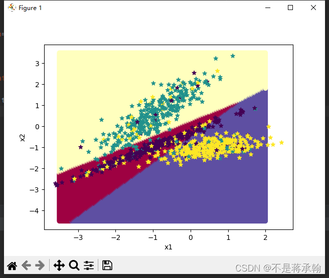

3.3 实践：基于Softmax回归完成鸢尾花分类任务

在本节，我们用入门深度学习的基础实验之一“鸢尾花分类任务”来进行实践，使用经典学术数据集Iris作为训练数据，实现基于Softmax回归的鸢尾花分类任务。

实践流程主要包括以下7个步骤：数据处理、模型构建、损失函数定义、优化器构建、模型训练、模型评价和模型预测等，

• 数据处理：根据网络接收的数据格式，完成相应的预处理操作，保证模型正常读取；
• 模型构建：定义Softmax回归模型类；
• 训练配置：训练相关的一些配置，如：优化算法、评价指标等；
• 组装Runner类：Runner用于管理模型训练和测试过程；
• 模型训练和测试：利用Runner进行模型训练、评价和测试。

3.3.1 数据处理

3.3.1.1 数据集介绍

Iris数据集，也称为鸢尾花数据集，包含了3种鸢尾花类别（Setosa、Versicolour、Virginica），每种类别有50个样本，共计150个样本。其中每个样本中包含了4个属性：花萼长度、花萼宽度、花瓣长度以及花瓣宽度，本实验通过鸢尾花这4个属性来判断该样本的类别。

3.3.1.2 数据清洗

• 缺失值分析

from sklearn.datasets import load_iris
import pandas
import numpy as np

iris_features = np.array(load_iris().data, dtype=np.float32)
iris_labels = np.array(load_iris().target, dtype=np.int32)
print(pandas.isna(iris_features).sum())
print(pandas.isna(iris_labels).sum())

0
0

从输出结果看，鸢尾花数据集中不存在缺失值的情况。

• 异常值处理

通过箱线图直观的显示数据分布，并观测数据中的异常值。

import matplotlib.pyplot as plt #可视化工具

# 箱线图查看异常值分布
def boxplot(features):
    feature_names = ['sepal_length', 'sepal_width', 'petal_length', 'petal_width']

    # 连续画几个图片
    plt.figure(figsize=(5, 5), dpi=200)
    # 子图调整
    plt.subplots_adjust(wspace=0.6)
    # 每个特征画一个箱线图
    for i in range(4):
        plt.subplot(2, 2, i+1)
        # 画箱线图
        plt.boxplot(features[:, i], 
                    showmeans=True, 
                    whiskerprops={"color":"#E20079", "linewidth":0.4, 'linestyle':"--"},
                    flierprops={"markersize":0.4},
                    meanprops={"markersize":1})
        # 图名
        plt.title(feature_names[i], fontdict={"size":5}, pad=2)
        # y方向刻度
        plt.yticks(fontsize=4, rotation=90)
        plt.tick_params(pad=0.5)
        # x方向刻度
        plt.xticks([])
    plt.savefig('ml-vis.pdf')
    plt.show()

boxplot(iris_features)

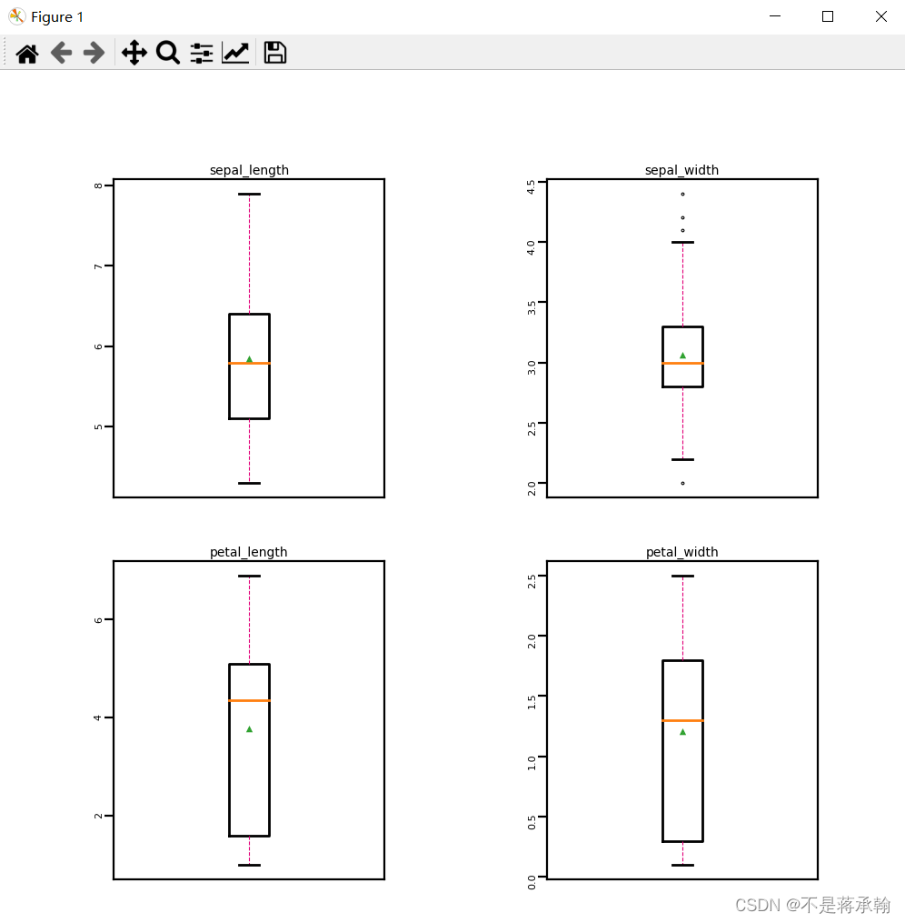
?从输出结果看，数据中基本不存在异常值，所以不需要进行异常值处理。

3.3.1.3 数据读取

本实验中将数据集划分为了三个部分：

• 训练集：用于确定模型参数；
• 验证集：与训练集独立的样本集合，用于使用提前停止策略选择最优模型；
• 测试集：用于估计应用效果（没有在模型中应用过的数据，更贴近模型在真实场景应用的效果）。

在本实验中，将80%的数据用于模型训练，10%的数据用于模型验证，10%的数据用于模型测试。代码实现如下：

import copy
import torch 

# 加载数据集
def load_data(shuffle=True):
    """
    加载鸢尾花数据
    输入：
        - shuffle：是否打乱数据，数据类型为bool
    输出：
        - X：特征数据，shape=[150,4]
        - y：标签数据, shape=[150]
    """
    # 加载原始数据
    X = np.array(load_iris().data, dtype=np.float32)
    y = np.array(load_iris().target, dtype=np.int32)

    X = torch.tensor(X)
    y = torch.tensor(y)

    # 数据归一化
    X_min = torch.min(X, dim=0)[0]
    X_max = torch.max(X, dim=0)[0]
    X = (X-X_min) / (X_max-X_min)

    # 如果shuffle为True，随机打乱数据
    if shuffle:
        idx = torch.randperm(X.shape[0])
        X = X[idx]
        y = y[idx]
    return X, y

# 固定随机种子
torch.manual_seed(102)

num_train = 120
num_dev = 15
num_test = 15

X, y = load_data(shuffle=True)
print("X shape: ", X.shape, "y shape: ", y.shape)
X_train, y_train = X[:num_train], y[:num_train]
X_dev, y_dev = X[num_train:num_train + num_dev], y[num_train:num_train + num_dev]
X_test, y_test = X[num_train + num_dev:], y[num_train + num_dev:]

X shape: ?torch.Size([150, 4]) y shape: ?torch.Size([150])

# 打印X_train和y_train的维度
print("X_train shape: ", X_train.shape, "y_train shape: ", y_train.shape)

X_train shape: ?torch.Size([120, 4]) y_train shape: ?torch.Size([120])

# 打印前5个数据的标签
print(y_train[:5])

tensor([1, 2, 0, 1, 2], dtype=torch.int32)

3.3.2 模型构建

使用Softmax回归模型进行鸢尾花分类实验，将模型的输入维度定义为4，输出维度定义为3。代码实现如下：

# 输入维度
input_dim = 4
# 类别数
output_dim = 3
# 实例化模型
model = model_SR(input_dim=input_dim, output_dim=output_dim)

3.3.3 模型训练

实例化RunnerV2类，使用训练集和验证集进行模型训练，共训练80个epoch，其中每隔10个epoch打印训练集上的指标，并且保存准确率最高的模型作为最佳模型。代码实现如下：

# 学习率
lr = 0.2

# 梯度下降法
optimizer = SimpleBatchGD(init_lr=lr, model=model)
# 交叉熵损失
loss_fn = MultiCrossEntropyLoss()
# 准确率
metric = accuracy

# 实例化RunnerV2
runner = RunnerV2(model, optimizer, metric, loss_fn)

# 启动训练
runner.train([X_train, y_train], [X_dev, y_dev], num_epochs=200, log_epochs=10, save_path="best_model.pdparams")

best accuracy performence has been updated: 0.00000 --> 0.46667
[Train] epoch: 0, loss: 1.09861159324646, score: 0.375
[Dev] epoch: 0, loss: 1.089357614517212, score: 0.46666666865348816
[Train] epoch: 10, loss: 0.9777261018753052, score: 0.699999988079071
[Dev] epoch: 10, loss: 1.023618221282959, score: 0.46666666865348816
[Train] epoch: 20, loss: 0.8894370794296265, score: 0.699999988079071
[Dev] epoch: 20, loss: 0.9739664793014526, score: 0.46666666865348816
[Train] epoch: 30, loss: 0.8196598291397095, score: 0.699999988079071
[Dev] epoch: 30, loss: 0.9317176938056946, score: 0.46666666865348816
[Train] epoch: 40, loss: 0.7635203003883362, score: 0.699999988079071
[Dev] epoch: 40, loss: 0.8957117199897766, score: 0.46666666865348816
[Train] epoch: 50, loss: 0.7176517248153687, score: 0.7250000238418579
[Dev] epoch: 50, loss: 0.864996075630188, score: 0.46666666865348816
[Train] epoch: 60, loss: 0.679577648639679, score: 0.7416666746139526
[Dev] epoch: 60, loss: 0.8386644721031189, score: 0.46666666865348816
[Train] epoch: 70, loss: 0.6474865078926086, score: 0.7583333253860474
[Dev] epoch: 70, loss: 0.8159360289573669, score: 0.46666666865348816
[Train] epoch: 80, loss: 0.6200525760650635, score: 0.7666666507720947
[Dev] epoch: 80, loss: 0.7961668372154236, score: 0.46666666865348816
[Train] epoch: 90, loss: 0.5962967276573181, score: 0.7833333611488342
[Dev] epoch: 90, loss: 0.7788369655609131, score: 0.46666666865348816
[Train] epoch: 100, loss: 0.5754876732826233, score: 0.8166666626930237
[Dev] epoch: 100, loss: 0.7635290622711182, score: 0.46666666865348816
best accuracy performence has been updated: 0.46667 --> 0.53333
[Train] epoch: 110, loss: 0.5570722222328186, score: 0.824999988079071
[Dev] epoch: 110, loss: 0.7499087452888489, score: 0.5333333611488342
best accuracy performence has been updated: 0.53333 --> 0.60000
[Train] epoch: 120, loss: 0.5406263470649719, score: 0.824999988079071
[Dev] epoch: 120, loss: 0.7377070188522339, score: 0.6000000238418579
[Train] epoch: 130, loss: 0.525819718837738, score: 0.8500000238418579
[Dev] epoch: 130, loss: 0.726706862449646, score: 0.6000000238418579
[Train] epoch: 140, loss: 0.5123931169509888, score: 0.8583333492279053
[Dev] epoch: 140, loss: 0.716731607913971, score: 0.6000000238418579
[Train] epoch: 150, loss: 0.5001395344734192, score: 0.875
[Dev] epoch: 150, loss: 0.7076371312141418, score: 0.6000000238418579
best accuracy performence has been updated: 0.60000 --> 0.66667
[Train] epoch: 160, loss: 0.4888923764228821, score: 0.875
[Dev] epoch: 160, loss: 0.6993042826652527, score: 0.6666666865348816
[Train] epoch: 170, loss: 0.4785163700580597, score: 0.875
[Dev] epoch: 170, loss: 0.6916342973709106, score: 0.6666666865348816
[Train] epoch: 180, loss: 0.46889936923980713, score: 0.875
[Dev] epoch: 180, loss: 0.6845448613166809, score: 0.6000000238418579
[Train] epoch: 190, loss: 0.45994895696640015, score: 0.875
[Dev] epoch: 190, loss: 0.6779663562774658, score: 0.6000000238418579

可视化观察训练集与验证集的准确率变化情况。

?

3.3.4 模型评价

使用测试数据对在训练过程中保存的最佳模型进行评价，观察模型在测试集上的准确率情况。代码实现如下：

# 加载最优模型
runner.load_model('best_model.pdparams')
# 模型评价
score, loss = runner.evaluate([X_test, y_test])
print("[Test] score/loss: {:.4f}/{:.4f}".format(score, loss))

?[Test] score/loss: 0.7333/0.5928

调整学习率为0.5后：

[Test] score/loss: 0.8667/0.4477

发现score上升，loss下降，

调整学习率为0.01后：

[Test] score/loss: 0.6000/1.0979

此结果和logistic回归类似，小的学习率收敛慢，还会过拟合将loss值升高。

调整epoch为5000后：

[Test] score/loss: 0.9333/0.2399

发现score明显上升，loss明显下降

调整epoch为10000后：

[Test] score/loss: 0.9333/0.2399

发现score和loss较50000没有改变

此时模型与logistic回归不同，没有发生过拟合。

3.3.5 模型预测

使用保存好的模型，对测试集中的数据进行模型预测，并取出1条数据观察模型效果。代码实现如下：

# 预测测试集数据
logits = runner.predict(X_test)
# 观察其中一条样本的预测结果
pred = torch.argmax(logits[0]).numpy()
# 获取该样本概率最大的类别
label = y_test[0].numpy()
# 输出真实类别与预测类别
print("The true category is {} and the predicted category is {}".format(label, pred))

The true category is 2 and the predicted category is 2

3.4 SVM训练Iris

分别使用线性核、多项式核与高斯核对Iris数据集的2/3数据训练支持向量机，剩余1/3数据进行测试，计算正确率。

import math  # 数学
import random  # 随机
import numpy as np
import matplotlib.pyplot as plt


def zhichi_w(zhichi, xy, a):  # 计算更新 w
    w = [0, 0]
    if len(zhichi) == 0:  # 初始化的0
        return w
    for i in zhichi:
        w[0] += a[i] * xy[0][i] * xy[2][i]  # 更新w
        w[1] += a[i] * xy[1][i] * xy[2][i]
    return w


def zhichi_b(zhichi, xy, a):  # 计算更新 b
    b = 0
    if len(zhichi) == 0:  # 初始化的0
        return 0
    for s in zhichi:  # 对任意的支持向量有 ysf(xs)=1 所有支持向量求解平均值
        sum = 0
        for i in zhichi:
            sum += a[i] * xy[2][i] * (xy[0][i] * xy[0][s] + xy[1][i] * xy[1][s])
        b += 1 / xy[2][s] - sum
    return b / len(zhichi)


def SMO(xy, m):
    a = [0.0] * len(xy[0])  # 拉格朗日乘子
    zhichi = set()  # 支持向量下标
    loop = 1  # 循环标记（符合KKT）
    w = [0, 0]  # 初始化 w
    b = 0  # 初始化 b
    while loop:
        loop += 1
        if loop == 150:
            print("达到早停标准")
            print("循环了：", loop, "次")
            loop = 0
            break
        # 初始化=========================================
        fx = []  # 储存所有的fx
        yfx = []  # 储存所有yfx-1的值
        Ek = []  # Ek,记录fx-y用于启发式搜索
        E_ = -1  # 贮存最大偏差，减少计算
        a1 = 0  # SMO  a1
        a2 = 0  # SMO  a2
        # 初始化结束======================================
        # 寻找a1,a2======================================
        for i in range(len(xy[0])):  # 计算所有的 fx yfx-1 Ek
            fx.append(w[0] * xy[0][i] + w[1] * xy[1][i] + b)  # 计算 fx=wx+b
            yfx.append(xy[2][i] * fx[i] - 1)  # 计算 yfx-1
            Ek.append(fx[i] - xy[2][i])  # 计算 fx-y
            if i in zhichi:  # 之前看过的不看了，防止重复找某个a
                continue
            if yfx[i] <= yfx[a1]:
                a1 = i  # 得到偏离最大位置的下标(数值最小的)
        if yfx[a1] >= 0:  # 最小的也满足KKT
            print("循环了：", loop, "次")
            loop = 0  # 循环标记（符合KKT）置零(没有用到)
            break
        for i in range(len(xy[0])):  # 遍历找间隔最大的a2
            if i == a1:  # 如果是a1，跳过
                continue
            Ei = abs(Ek[i] - Ek[a1])  # |Eki-Eka1|
            if Ei < E_:  # 找偏差
                E_ = Ei  # 储存偏差的值
                a2 = i  # 储存偏差的下标
        # 寻找a1,a2结束===================================
        zhichi.add(a1)  # a1录入支持向量
        zhichi.add(a2)  # a2录入支持向量
        # 分析约束条件=====================================
        # c=a1*y1+a2*y2
        c = a[a1] * xy[2][a1] + a[a2] * xy[2][a2]  # 求出c
        # n=K11+k22-2*k12
        if m == "xianxinghe":  # 线性核
            n = xy[0][a1] ** 2 + xy[1][a1] ** 2 + xy[0][a2] ** 2 + xy[1][a2] ** 2 - 2 * (
                    xy[0][a1] * xy[0][a2] + xy[1][a1] * xy[1][a2])
        elif m == "duoxiangshihe":  # 多项式核(这里是二次)
            n = (xy[0][a1] ** 2 + xy[1][a1] ** 2) ** 2 + (xy[0][a2] ** 2 + xy[1][a2] ** 2) ** 2 - 2 * (
                    xy[0][a1] * xy[0][a2] + xy[1][a1] * xy[1][a2]) ** 2
        else:  # 高斯核  取 2σ^2 = 1
            n = 2 * math.exp(-1) - 2 * math.exp(-((xy[0][a1] - xy[0][a2]) ** 2 + (xy[1][a1] - xy[1][a2]) ** 2))
        # 确定a1的可行域=====================================
        if xy[2][a1] == xy[2][a2]:
            L = max(0.0, a[a1] + a[a2] - 0.5)  # 下界
            H = min(0.5, a[a1] + a[a2])  # 上界
        else:
            L = max(0.0, a[a1] - a[a2])  # 下界
            H = min(0.5, 0.5 + a[a1] - a[a2])  # 上界
        if n > 0:
            a1_New = a[a1] - xy[2][a1] * (Ek[a1] - Ek[a2]) / n  # a1_New = a1_old-y1(e1-e2)/n
            # print("x1=",xy[0][a1],"y1=",xy[1][a1],"z1=",xy[2][a1],"x2=",xy[0][a2],"y2=",xy[1][a2],"z2=",xy[2][a2],"a1_New=",a1_New)
            # 越界裁剪============================================================
            if a1_New >= H:
                a1_New = H
            elif a1_New <= L:
                a1_New = L
        else:
            a1_New = min(H, L)
        # 参数更新=======================================
        a[a2] = a[a2] + xy[2][a1] * xy[2][a2] * (a[a1] - a1_New)  # a2更新
        a[a1] = a1_New  # a1更新
        w = zhichi_w(zhichi, xy, a)  # 更新w
        b = zhichi_b(zhichi, xy, a)  # 更新b
        # print("W=", w, "b=", b, "zhichi=", zhichi, "a1=", a[a1], "a2=", a[a2])
    # 标记支持向量======================================
    for i in zhichi:
        if a[i] == 0:  # 选了，但值仍为0
            loop = loop + 1
            e = 'silver'
        else:
            if xy[2][i] == 1:
                e = 'b'
            else:
                e = 'r'
        plt.scatter(x1[0][i], x1[1][i], c='none', s=100, linewidths=1, edgecolor=e)
    print("支持向量数为：", len(zhichi), "\na为零支持向量：", loop)
    print("有用向量数：", len(zhichi) - loop)
    # 返回数据 w b =======================================
    return [w, b]


def panduan(xyz, w_b1, w_b2):
    c = 0
    for i in range(len(xyz[0])):
        if (xyz[0][i] * w_b1[0][0] + xyz[1][i] * w_b1[0][1] + w_b1[1]) * xyz[2][i][0] < 0:
            c = c + 1
            continue
        if (xyz[0][i] * w_b2[0][0] + xyz[1][i] * w_b2[0][1] + w_b2[1]) * xyz[2][i][1] < 0:
            c = c + 1
            continue
    return (1 - c / len(xyz[0])) * 100


def huitu(x1, x2, wb1, wb2, name):
    x = [x1[0][:], x1[1][:], x1[2][:]]
    for i in range(len(x[2])):  # 对训练集‘上色’
        if x[2][i] == [1, 1]:
            x[2][i] = 'r'  # 训练集  1  1 红色
        elif x[2][i] == [-1, 1]:
            x[2][i] = 'g'  # 训练集 -1  1 绿色
        else:
            x[2][i] = 'b'  # 训练集 -1 -1 蓝色
    plt.scatter(x[0], x[1], c=x[2], alpha=0.8)  # 绘点训练集
    x = [x2[0][:], x2[1][:], x2[2][:]]
    for i in range(len(x[2])):  # 对测试集‘上色’
        if x[2][i] == [1, 1]:
            x[2][i] = 'orange'  # 训练集  1   1 橙色
        elif x[2][i] == [-1, 1]:
            x[2][i] = 'y'  # 训练集 -1   1 黄色
        else:
            x[2][i] = 'm'  # 训练集 -1  -1 紫色
    plt.scatter(x[0], x[1], c=x[2], alpha=0.8)  # 绘点测试集
    plt.xlabel('x')  # x轴标签
    plt.ylabel('y')  # y轴标签
    plt.title(name)  # 标题
    xl = np.arange(min(x[0]), max(x[0]), 0.1)  # 绘制分类线一
    yl = (-wb1[0][0] * xl - wb1[1]) / wb1[0][1]
    plt.plot(xl, yl, 'r')
    xl = np.arange(min(x[0]), max(x[0]), 0.1)  # 绘制分类线二
    yl = (-wb2[0][0] * xl - wb2[1]) / wb2[0][1]
    plt.plot(xl, yl, 'b')


# 主函数=======================================================
f = open('Iris.txt', 'r')  # 读文件
x = [[], [], [], [], []]  # 花朵属性，(0,1,2,3),花朵种类
while 1:
    yihang = f.readline()  # 读一行
    if len(yihang) <= 1:  # 读到末尾结束
        break
    fenkai = yihang.split('\t')  # 按\t分开
    for i in range(4):  # 分开的四个值
        x[i].append(eval(fenkai[i]))  # 化为数字加到x中
    if (eval(fenkai[4]) == 1):  # 将标签化为向量形式
        x[4].append([1, 1])
    else:
        if (eval(fenkai[4]) == 2):
            x[4].append([-1, 1])
        else:
            x[4].append([-1, -1])

print('数据集=======================================================')
print(len(x[0]))  # 数据大小
# 选择数据===================================================
shuxing1 = eval(input("选取第一个属性："))
if shuxing1 < 0 or shuxing1 > 4:
    print("无效选项，默认选择第1项")
    shuxing1 = 1
shuxing2 = eval(input("选取第一个属性："))
if shuxing2 < 0 or shuxing2 > 4 or shuxing1 == shuxing2:
    print("无效选项，默认选择第2项")
    shuxing2 = 2
# 生成数据集==================================================
lt = list(range(150))  # 得到一个顺序序列
random.shuffle(lt)  # 打乱序列
x1 = [[], [], []]  # 初始化x1
x2 = [[], [], []]  # 初始化x2
for i in lt[0:100]:  # 截取部分做训练集
    x1[0].append(x[shuxing1][i])  # 加上数据集x属性
    x1[1].append(x[shuxing2][i])  # 加上数据集y属性
    x1[2].append(x[4][i])  # 加上数据集c标签
for i in lt[100:150]:  # 截取部分做测试集
    x2[0].append(x[shuxing1][i])  # 加上数据集x属性
    x2[1].append(x[shuxing2][i])  # 加上数据集y属性
    x2[2].append(x[4][i])  # 加上数据集c标签
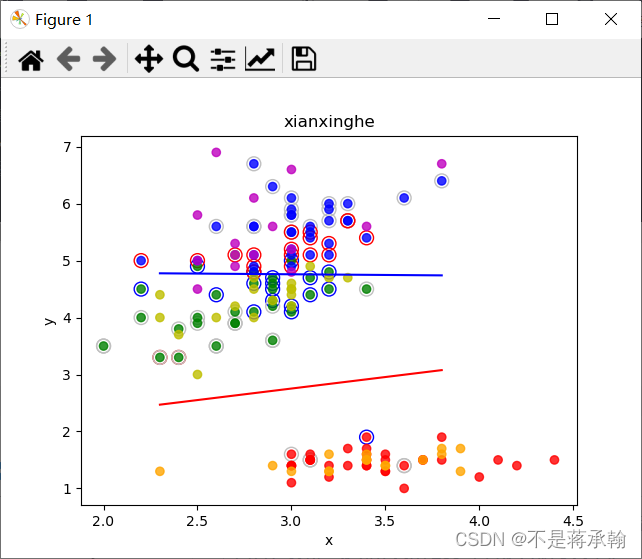
print('\n\n开始训练==============================================')
print('\n线性核==============================================')
# 计算 w b============================================
plt.figure(1)  # 第一张画布
x = [x1[0][:], x1[1][:], []]  # 第一次分类
for i in x1[2]:
    x[2].append(i[0])  # 加上数据集标签
wb1 = SMO(x, "xianxinghe")
x = [x1[0][:], x1[1][:], []]  # 第二次分类
for i in x1[2]:
    x[2].append(i[1])  # 加上数据集标签
wb2 = SMO(x, "xianxinghe")
print("w1为：", wb1[0], " b1为：", wb1[1])
print("w2为：", wb2[0], " b2为：", wb2[1])
# 计算正确率===========================================
print("训练集上的正确率为：", panduan(x1, wb1, wb2), "%")
print("测试集上的正确率为：", panduan(x2, wb1, wb2), "%")
# 绘图 ===============================================
# 圈着的是曾经选中的值，灰色的是选中但更新为0
huitu(x1, x2, wb1, wb2, "xianxinghe")
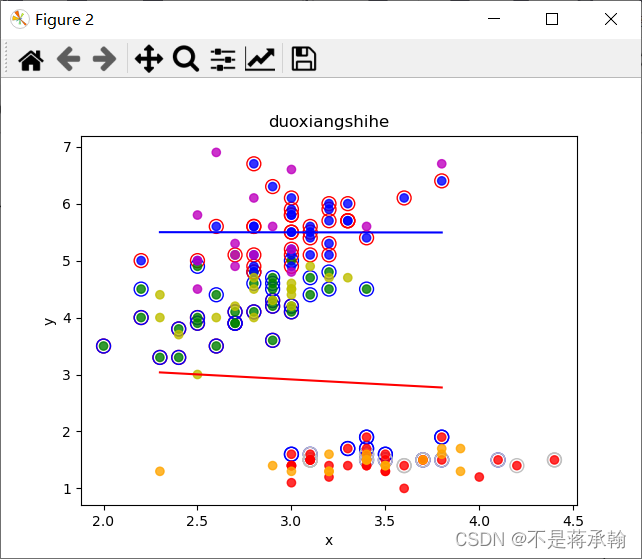
print('\n多项式核============================================')
# 计算 w b============================================
plt.figure(2)  # 第二张画布
x = [x1[0][:], x1[1][:], []]  # 第一次分类
for i in x1[2]:
    x[2].append(i[0])  # 加上数据集标签
wb1 = SMO(x, "duoxiangshihe")
x = [x1[0][:], x1[1][:], []]  # 第二次分类
for i in x1[2]:
    x[2].append(i[1])  # 加上数据集标签
wb2 = SMO(x, "duoxiangshihe")
print("w1为：", wb1[0], " b1为：", wb1[1])
print("w2为：", wb2[0], " b2为：", wb2[1])
# 计算正确率===========================================
print("训练集上的正确率为：", panduan(x1, wb1, wb2), "%")
print("测试集上的正确率为：", panduan(x2, wb1, wb2), "%")
# 绘图 ===============================================
# 圈着的是曾经选中的值，灰色的是选中但更新为0
huitu(x1, x2, wb1, wb2, "duoxiangshihe")
print('\n高斯核==============================================')
# 计算 w b============================================
plt.figure(3)  # 第三张画布
x = [x1[0][:], x1[1][:], []]  # 第一次分类
for i in x1[2]:
    x[2].append(i[0])  # 加上数据集标签
wb1 = SMO(x, "gaosihe")
x = [x1[0][:], x1[1][:], []]  # 第二次分类
for i in x1[2]:
    x[2].append(i[1])  # 加上数据集标签
wb2 = SMO(x, "gaosihe")
print("w1为：", wb1[0], " b1为：", wb1[1])
print("w2为：", wb2[0], " b2为：", wb2[1])
# 计算正确率===========================================
print("训练集上的正确率为：", panduan(x1, wb1, wb2), "%")
print("测试集上的正确率为：", panduan(x2, wb1, wb2), "%")
# 绘图 ===============================================
# 圈着的是曾经选中的值，灰色的是选中但更新为0
huitu(x1, x2, wb1, wb2, "gaosihe")
# 显示所有图
plt.show()  # 显示

?

线性核==============================================
循环了： 13 次
支持向量数为： 12?
a为零支持向量： 7
有用向量数： 5
循环了： 69 次
支持向量数为： 68?
a为零支持向量： 31
有用向量数： 37
w1为： [0.3172050400916382, -0.903111111111111] ?b1为： 1.423599618174875
w2为： [0.13003047759163255, -0.48005708869482205] ?b2为： 1.9588662762259441
训练集上的正确率为： 97.0 %
测试集上的正确率为： 94.0 %

多项式核============================================
达到早停标准
循环了： 150 次
支持向量数为： 58?
a为零支持向量： 6
有用向量数： 52
达到早停标准
循环了： 150 次
支持向量数为： 88?
a为零支持向量： 16
有用向量数： 72
w1为： [-0.15104036408342042, -0.42676907221895527] ?b1为： 1.7115652617123134
w2为： [0.0016951361729040434, -0.1288161548404545] ?b2为： 0.7522268880681302
训练集上的正确率为： 75.0 %
测试集上的正确率为： 74.0 %

高斯核==============================================
循环了： 6 次
支持向量数为： 5?
a为零支持向量： 3
有用向量数： 2
循环了： 68 次
支持向量数为： 67?
a为零支持向量： 57
有用向量数： 10
w1为： [-0.15000000000000013, -1.55] ?b1为： 4.604000000000001
w2为： [0.21169007613908675, -0.5635355081003279] ?b2为： 2.129028885189375
训练集上的正确率为： 97.0 %
测试集上的正确率为： 92.0 %

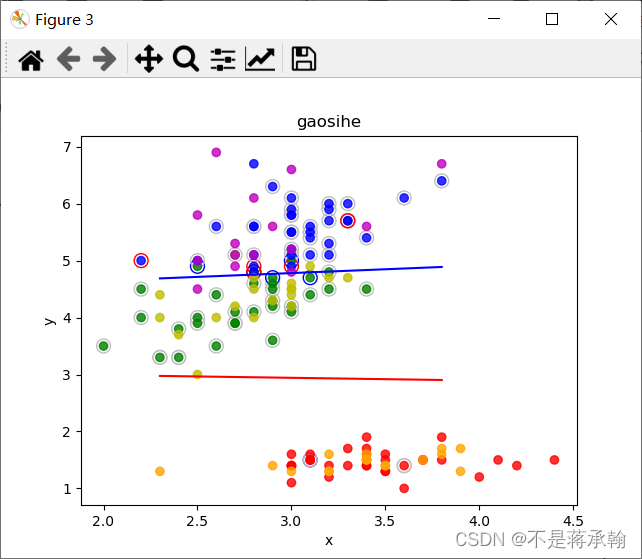
?SVM的精度与训练50000epoch的softmax分类模型差不多。

?心得体会：

本次实验还是对上学期机器学习内容的复习，把上次实验的线性回归模型放在一起比较，

总的来说两个问题本质上都是一致的，就是模型的拟合（匹配）。 但是分类问题的y值(也称为label), 更离散化一些，而且， 同一个y值可能对应着一大批的x，这些x是具有一定范围的。?
所以分类问题更多的是 (一定区域的一些x) 对应 着 (一个y)。而回归问题的模型更倾向于 (很小区域内的x，或者一般是一个x) ?对应着 ?(一个y)，分类模型是将回归模型的输出离散化。

所以在把一个问题建模的时候一定要考虑好需求，让你的模型更好的与现实问题相对应。

本次实验还有一处问题是超参数的选择，如何选择学习率和训练轮数可以使模型精度更高，模型训练的时候一般把epoch设置多大达到模型收敛，如何设置动态学习率，这些问题都要在实验后继续研究。

这次写实验也是查阅了好多资料，抱着西瓜书、蒲公英书、鱼书一起看，电脑cpu没冒烟，我脑袋先冒烟了。