[人工智能]机器学习实战（10）——Tensorflow

CSDN话题挑战赛第2期
参赛话题：学习笔记

目录

1 TensorFlow中的线性回归

module 'tensorflow' has no attribute 'xxx'解决方案

2 梯度下降的实现

2.1 手工计算梯度

2.2 使用自动微分

2.3 使用优化器

3 给训练算法提供数据

4 保存和恢复模型

5 用TensorBoard来可视化图和训练曲线

供参考：开始 (juejin.im)

有关?tensorflow 参考文档可以在上述网站下载。

一个Tensorflow程序通常可以分成两个部分：第一部分用来构建一个计算图（称为构建阶段），第二部分来执行这个图（称为执行阶段）。构建阶段通常会构建一个计算图，这个图用来展现ML模型和训练所需的计算。执行阶段则重复地执行每一步训练动作，并逐步提升模型的参数。

在此我们使用jupyter进行演练，如果你还没有下载安装tensorflow，可以使用下面代码实现：

pip install tensorflow -i https://pypi.tuna.tsinghua.edu.cn/simple

常规模块导入及可视化设置：

# Common imports
import numpy as np
import os

# 结果复现，随机数种子
def reset_graph(seed=42):
    tf.compat.v1.reset_default_graph() #tensorflow2.0以上版本需要tf.compat.v1作为接口
    tf.compat.v1.set_random_seed(seed)
    np.random.seed(seed)

# To plot pretty figures
import matplotlib
import matplotlib.pyplot as plt
plt.rcParams['axes.labelsize'] = 14
plt.rcParams['xtick.labelsize'] = 12
plt.rcParams['ytick.labelsize'] = 12

1 TensorFlow中的线性回归

输入和输出都是多维数组的话，叫做张量。之前我们演示的代码中，张量都只包含了单个标量值，但可以对任意形状的数组进行计算。

下面的代码展示了如何操作二维的数组来计算加州的住房数据的线性回归。首先，获取数据。然后，对所有训练实例都添加一个额外的偏移。接下来，创建两个TensorFlow的常量节点，x和y以及目标（标签，注意housing.target是一个一维数组，我们需要将它变成一个列向量再来计算）。

module 'tensorflow' has no attribute 'xxx'解决方案

你也可以选择略过该部分，如果你是初次使用tf请留步：

有关module 'tensorflow' has no attribute 'xxx'可以参考：

关于tensorflow 中module ‘tensorflow‘ has no attribute ‘xxx‘问题的根本解决方法。_进击的炼丹师的博客-CSDN博客

tensorflow张量和numpy数组相互转换，参考：

??????tensorflow张量和numpy数组相互转换_新诺斯给的博客-CSDN博客_tf转numpy

代码展示：

注意：tensorflow2.0以上版本需要tf.compat.v1作为接口

因此，我们可以这样导入：

import tenforflow.compat.v1 as tf

不过，下面为了体现接口，我依然是使用以下导入：

import tenforflow as tf

eager_execution 是tensorflow的立即执行模式，在2.x的tensorflow版本中是默认打开，我们需要调用tf.compat.v1.disable_eager_execution()去关闭。

如果不关闭该模式，则需要.numpy()来转换成数组，继续用eval()则会报错：

用tf.compat.v1.disable_eager_execution()去关闭：

import numpy as np
from sklearn.datasets import fetch_california_housing

reset_graph()
tf.compat.v1.disable_eager_execution()

#加载数据
housing = fetch_california_housing()
m, n = housing.data.shape

#偏移
housing_data_plus_bias = np.c_[np.ones((m, 1)), housing.data]

#创建两个常量节点
X = tf.constant(housing_data_plus_bias, dtype=tf.float32, name="X")
y = tf.constant(housing.target.reshape(-1, 1), dtype=tf.float32, name="y")

#转置
XT = tf.transpose(X) #transpose()为tf内置矩阵函数（转置），下同

#正规方程
#下面tf.matmul(a,b) #矩阵ab相乘

theta = tf.matmul(tf.matmul(tf.compat.v1.matrix_inverse(tf.matmul(XT, X)), XT), y)

#使用with，也就是python的上下文管理器，执行会会自动关闭会话，释放内存，简单高效！
with tf.compat.v1.Session() as sess:
    theta_value = theta.eval() #与tf.compat.v1.disable_eager_execution()呼应
    
theta_value

用.numpy()来转换成数组：

import numpy as np
from sklearn.datasets import fetch_california_housing

reset_graph()

housing = fetch_california_housing()
m, n = housing.data.shape
housing_data_plus_bias = np.c_[np.ones((m, 1)), housing.data]

X = tf.constant(housing_data_plus_bias, dtype=tf.float32, name="X")
y = tf.constant(housing.target.reshape(-1, 1), dtype=tf.float32, name="y")
XT = tf.transpose(X)
theta = tf.matmul(tf.matmul(tf.compat.v1.matrix_inverse(tf.matmul(XT, X)), XT), y)

with tf.compat.v1.Session() as sess:
    theta_value = theta.numpy()
    
theta_value

运行后你会发现，两个结果是一样的：

array([[-3.68901253e+01],
       [ 4.36643779e-01],
       [ 9.45042260e-03],
       [-1.07117996e-01],
       [ 6.43712580e-01],
       [-3.96291580e-06],
       [-3.78801115e-03],
       [-4.20931637e-01],
       [-4.34006572e-01]], dtype=float32)

我们之前?numpy 是这样计算?theta_value：

X = housing_data_plus_bias
y = housing.target.reshape(-1, 1)
theta_numpy = np.linalg.inv(X.T.dot(X)).dot(X.T).dot(y)

theta_numpy

运行结果如下：

array([[-3.69419202e+01],
       [ 4.36693293e-01],
       [ 9.43577803e-03],
       [-1.07322041e-01],
       [ 6.45065693e-01],
       [-3.97638942e-06],
       [-3.78654265e-03],
       [-4.21314378e-01],
       [-4.34513755e-01]])

当然我们可以线性回归：

from sklearn.linear_model import LinearRegression
lin_reg = LinearRegression()
lin_reg.fit(housing.data, housing.target.reshape(-1, 1))

np.r_[lin_reg.intercept_.reshape(-1, 1), lin_reg.coef_.T]

运行结果如下：

[[-3.69419202e+01]
 [ 4.36693293e-01]
 [ 9.43577803e-03]
 [-1.07322041e-01]
 [ 6.45065694e-01]
 [-3.97638942e-06]
 [-3.78654265e-03]
 [-4.21314378e-01]
 [-4.34513755e-01]]

2 梯度下降的实现

当使用梯度下降时，我们首先需要对输入的特征向量做归一化处理。

2.1 手工计算梯度

#归一化处理
from sklearn.preprocessing import StandardScaler
scaler = StandardScaler()
scaled_housing_data = scaler.fit_transform(housing.data)
scaled_housing_data_plus_bias = np.c_[np.ones((m, 1)), scaled_housing_data]


reset_graph() #随机数种子，便于结果复现

n_epochs = 1000 #训练步骤
learning_rate = 0.01 #学习率

X = tf.constant(scaled_housing_data_plus_bias, dtype=tf.float32, name="X")
y = tf.constant(housing.target.reshape(-1, 1), dtype=tf.float32, name="y")

#random_uniform()会在图中创建一个节点，这个节点会生成一个张量。此函数会根据传入的形状和值域来生成随机值来填充这个张量

theta = tf.Variable(tf.compat.v1.random_uniform([n + 1, 1], -1.0, 1.0, seed=42), name="theta")

y_pred = tf.matmul(X, theta, name="predictions")
error = y_pred - y
mse = tf.reduce_mean(tf.square(error), name="mse")
gradients = 2/m * tf.matmul(tf.transpose(X), error)

#通过assign()创建一个为变量赋值的节点。下面实现的是批量梯度下降
training_op = tf.compat.v1.assign(theta, theta - learning_rate * gradients)

init = tf.compat.v1.global_variables_initializer()#看下面讲解

with tf.compat.v1.Session() as sess:
    sess.run(init)

    for epoch in range(n_epochs):
        if epoch % 100 == 0:
            print("Epoch", epoch, "MSE =", mse.eval()) #主循环不断执行训练步骤（共n_epochs次），每经过100次迭代打印当前的均方差
        sess.run(training_op)
    
    best_theta = theta.eval()

运行结果如下：

Epoch 0 MSE = 9.161542
Epoch 100 MSE = 0.71450037
Epoch 200 MSE = 0.56670487
Epoch 300 MSE = 0.55557173
Epoch 400 MSE = 0.54881126
Epoch 500 MSE = 0.5436363
Epoch 600 MSE = 0.5396291
Epoch 700 MSE = 0.5365092
Epoch 800 MSE = 0.53406775
Epoch 900 MSE = 0.53214735

关于?tf.Variable()初始化和变量名可以参考：

[472]tf.Variable()函数_周小董的博客-CSDN博客_tf.variable

关于为什么使用 init = tf.compat.v1.global_variables_initializer() 初始化：

import tensorflow as tf
# 必须要使用global_variables_initializer的场合
# 含有tf.Variable的环境下，因为tf中建立的变量是没有初始化的，也就是在debug时还不是一个tensor量，而是一个Variable变量类型
size_out = 10
tensor = tf.Variable(tf.random_normal(shape=[size_out]))
init = tf.compat.v1.global_variables_initializer()
with tf.compat.v1.Session() as sess:
    sess.run(init)  # initialization variables
    print(sess.run(tensor))
# 可以不适用初始化的场合
# 不含有tf.Variable、tf.get_Variable的环境下
# 比如只有tf.random_normal或tf.constant等
size_out = 10
tensor = tf.random_normal(shape=[size_out])  # 这里debug是一个tensor量哦
init = tf.compat.v1.global_variables_initializer()
with tf.compat.v1.Session() as sess:
    # sess.run(init)  # initialization variables
    print(sess.run(tensor))

参考：tf.global_variables_initializer()什么时候用？_做一只AI小能手的博客-CSDN博客_tf.global_variables_initializer?

2.2 使用自动微分

上面的代码是使用数学的方式从成本函数（均方误差）中计算出梯度的。TensorFlow中的autodiff可以自动而且高效地算出梯度，只需要对例子中gradients的赋值的语句做出以下变化：

gradients = 2/m * tf.matmul(tf.transpose(X), error)

替换为：

gradients = tf.gradients(mse, [theta])[0]

gradients() 函数接受一个操作符（这里是mse）和一个参数列表（theta）作为参数，然后它会创建一个操作符的列表来计算每个变量的梯度。

运行结果不变：

Epoch 0 MSE = 9.161542
Epoch 100 MSE = 0.71450037
Epoch 200 MSE = 0.5667048
Epoch 300 MSE = 0.5555718
Epoch 400 MSE = 0.54881126
Epoch 500 MSE = 0.5436363
Epoch 600 MSE = 0.53962916
Epoch 700 MSE = 0.5365092
Epoch 800 MSE = 0.53406775
Epoch 900 MSE = 0.53214735

TensorFlow中的autodiff算法非常适合有多个输入和少量输出的场景，高效且精确。

2.3 使用优化器

同样我们可以使用梯度下降优化器。

我们需要将下面的代码：

gradients = tf.gradients(mse, [theta])[0]

training_op = tf.compat.v1.assign(theta, theta - learning_rate * gradients)

替换为：

optimizer = tf.compat.v1.train.GradientDescentOptimizer(learning_rate=learning_rate)
training_op = optimizer.minimize(mse)

运行结果如下：

Epoch 0 MSE = 9.161542
Epoch 100 MSE = 0.71450037
Epoch 200 MSE = 0.5667048
Epoch 300 MSE = 0.5555718
Epoch 400 MSE = 0.54881126
Epoch 500 MSE = 0.5436363
Epoch 600 MSE = 0.53962916
Epoch 700 MSE = 0.5365092
Epoch 800 MSE = 0.53406775
Epoch 900 MSE = 0.53214735

3 给训练算法提供数据

如果我们把上面的代码改成小批次梯度下降。为此，我们需要一种在每次迭代时用下一个小批量替换X和y的方法。我们一般用占位符节点在训练过程中将值传递给TensorFlow。占位符节点非常特别，它们不进行任何实际的计算，而只是在运行时输出我们需要它输出的值。如果运行时不为占位符指定一个值，就会得到异常。

创建一个占位符节点，需要调用placeholder()函数并制定输出张量的数据类型。我们可以指定张量的形状，如果设置None，表示“任意尺寸”。

例如，下面的代码创建一个占位符节点A，同时创建节点B，节点B=A+5。当对B求值时，给eval()方法传一个feed_dict，并制定A的值。

reset_graph()

A = tf.compat.v1.placeholder(tf.float32, shape=(None, 3))
B = A + 5
with tf.compat.v1.Session() as sess:
    B_val_1 = B.eval(feed_dict={A: [[1, 2, 3]]})
    B_val_2 = B.eval(feed_dict={A: [[4, 5, 6], [7, 8, 9]]})

print(B_val_1)
print(B_val_2)

运行结果如下：

[[6. 7. 8.]]

[[ 9. 10. 11.]
 [12. 13. 14.]]

那么如何实现小批次梯度下降？首先在构造阶段把X和y定义为占位符节点。

n_epochs = 1000 #训练步骤
learning_rate = 0.01 #学习率

reset_graph() #结果复现


#定义占位符节点
X = tf.compat.v1.placeholder(tf.float32, shape=(None, n + 1), name="X")
y = tf.compat.v1.placeholder(tf.float32, shape=(None, 1), name="y")

其他不变

theta = tf.Variable(tf.compat.v1.random_uniform([n + 1, 1], -1.0, 1.0, seed=42), name="theta")
y_pred = tf.matmul(X, theta, name="predictions")
error = y_pred - y
mse = tf.reduce_mean(tf.square(error), name="mse")
optimizer = tf.compat.v1.train.GradientDescentOptimizer(learning_rate=learning_rate)
training_op = optimizer.minimize(mse)

init = tf.compat.v1.global_variables_initializer()

下面定义批次的大小并计算批次的总数：

n_epochs = 10

batch_size = 100
n_batches = int(np.ceil(m / batch_size))

执行阶段，逐个获取小批次，然后在评估依赖于它们的节点时，通过feed_dict参数提供X和y的值。

def fetch_batch(epoch, batch_index, batch_size):
    np.random.seed(epoch * n_batches + batch_index)  # not shown in the book
    indices = np.random.randint(m, size=batch_size)  # not shown
    X_batch = scaled_housing_data_plus_bias[indices] # not shown
    y_batch = housing.target.reshape(-1, 1)[indices] # not shown
    return X_batch, y_batch

with tf.compat.v1.Session() as sess:
    sess.run(init)

    for epoch in range(n_epochs):
        for batch_index in range(n_batches):
            X_batch, y_batch = fetch_batch(epoch, batch_index, batch_size)
            sess.run(training_op, feed_dict={X: X_batch, y: y_batch})

    best_theta = theta.eval()


best_theta

运行结果如下：

array([[ 2.0703337 ],
       [ 0.8637145 ],
       [ 0.12255151],
       [-0.31211874],
       [ 0.38510373],
       [ 0.00434168],
       [-0.01232954],
       [-0.83376896],
       [-0.8030471 ]], dtype=float32)

4 保存和恢复模型

在构造期末尾（所有变量节点都创建之后）创建一个Saver节点，然后在执行期，调用save()方法，并传入一个会话和检查点文件的路径即可保存模型：

reset_graph()

n_epochs = 1000                                                                       # not shown in the book
learning_rate = 0.01                                                                  # not shown

X = tf.constant(scaled_housing_data_plus_bias, dtype=tf.float32, name="X")            # not shown
y = tf.constant(housing.target.reshape(-1, 1), dtype=tf.float32, name="y")            # not shown
theta = tf.Variable(tf.compat.v1.random_uniform([n + 1, 1], -1.0, 1.0, seed=42), name="theta")
y_pred = tf.matmul(X, theta, name="predictions")                                      # not shown
error = y_pred - y                                                                    # not shown
mse = tf.reduce_mean(tf.square(error), name="mse")                                    # not shown
optimizer = tf.compat.v1.train.GradientDescentOptimizer(learning_rate=learning_rate)            # not shown
training_op = optimizer.minimize(mse)                                                 # not shown

init = tf.compat.v1.global_variables_initializer()
saver = tf.compat.v1.train.Saver()

with tf.compat.v1.Session() as sess:
    sess.run(init)

    for epoch in range(n_epochs):
        if epoch % 100 == 0:
            print("Epoch", epoch, "MSE =", mse.eval())                                # not shown
            save_path = saver.save(sess, "E:/PYTHON/my_model.ckpt")
        sess.run(training_op)
    
    best_theta = theta.eval()
    save_path = saver.save(sess, "E:/PYTHON/my_model.ckpt")

运行结果如下：

Epoch 0 MSE = 9.161542
Epoch 100 MSE = 0.71450037
Epoch 200 MSE = 0.5667048
Epoch 300 MSE = 0.5555718
Epoch 400 MSE = 0.54881126
Epoch 500 MSE = 0.5436363
Epoch 600 MSE = 0.53962916
Epoch 700 MSE = 0.5365092
Epoch 800 MSE = 0.53406775
Epoch 900 MSE = 0.53214735

下面恢复模型，与之前一样，在构造期末尾创建一个Saver节点，不过在执行期开始的时候，不适用init节点来初始化变量，而是调用Saver对象上的restore()方法：

with tf.compat.v1.Session() as sess:
    saver.restore(sess, "E:/PYTHON/my_model.ckpt")
    best_theta_restored = theta.eval() # not shown in the book

运行结果如下：?

INFO:tensorflow:Restoring parameters from E:/PYTHON/my_model.ckpt

5 用TensorBoard来可视化图和训练曲线

首先要对程序稍作修改，这样它可以将图的定义和训练状态，比如，训练误差，写入到一个?TensorBoard 会读取的日志文件夹中。每次运行程序时，都需要指定一个不同的目录，否则TensorBoard会将这些状态信息合并起来，最简单的方式是用时间戳来命名日志文件。

把下面的代码放在程序的开始部分：

from datetime import datetime

now = datetime.utcnow().strftime("%Y%m%d%H%M%S")
root_logdir = "tf_logs"
logdir = "{}/run-{}/".format(root_logdir, now)

logdir

运行结果如下：

'tf_logs/run-20220923150948/'

实际上，我们可以创建一个函数，它将在每次需要时生成这样的子目录路径:?

def make_log_subdir(run_id=None):
    if run_id is None:
        run_id = datetime.utcnow().strftime("%Y%m%d%H%M%S")
    return "{}/run-{}/".format(root_logdir, run_id)

现在让我们使用tf.summary.FileWriter()将默认图形保存到log子目录:

file_writer = tf.compat.v1.summary.FileWriter(logdir, graph=tf.compat.v1.get_default_graph())

现在根日志目录包含一个子目录:

os.listdir(root_logdir)

运行结果如下：

['run-20220923150948']

这个子目录包含一个图的日志文件(称为“TF事件”文件):

os.listdir(logdir)

运行结果如下：

['events.out.tfevents.1616665937.kiwimac']

然而，实际的图形数据可能仍然在操作系统的文件缓存中，所以我们需要flush()或close()这个FileWriter，以确保它被很好地写入磁盘:?

file_writer.close()

现在让我们开始TensorBoard。它在一个单独的进程中作为web服务器运行，所以我们首先需要启动它。一种方法是在终端窗口中运行tensorboard命令。另一个是使用%tensorboard Jupyter扩展，它负责启动tensorboard，它允许我们直接在Jupyter中查看tensorboard的用户界面。现在让我们加载这个扩展:

%load_ext tensorboard

接下来，让我们使用%tensorboard扩展名来启动tensorboard服务器。我们需要将它指向根日志目录:

%tensorboard --logdir {root_logdir}

运行结果如下：?

ERROR: Timed out waiting for TensorBoard to start. It may still be running as pid 21256.

成功如下：

我们现在可以可视化图形。实际上，我们可以通过创建一个save_graph()函数来简化这个过程，该函数将自动创建一个新的日志子目录，并将给定的图(默认情况下是tf.get_default_graph())保存到这个目录:

def save_graph(graph=None, run_id=None):
    if graph is None:
        graph = tf.compat.v1.get_default_graph()
    logdir = make_log_subdir(run_id)
    file_writer = tf.compat.v1.summary.FileWriter(logdir, graph=graph)
    file_writer.close()
    return logdir

save_graph()

运行结果如下：?

'tf_logs/run-20220923153005/'

我们再来看看TensorBoard。注意，这将重用现有的TensorBoard服务器，因为我们重用的是相同的根日志目录:?

%tensorboard --logdir {root_logdir}

运行结果如下：?

注意，我们可以通过从“Run”下拉列表(在左上角)中选择您想要的日志子目录来切换运行。

现在让我们看看如何可视化学习曲线:

reset_graph()

n_epochs = 1000
learning_rate = 0.01

X = tf.compat.v1.placeholder(tf.float32, shape=(None, n + 1), name="X")
y = tf.compat.v1.placeholder(tf.float32, shape=(None, 1), name="y")
theta = tf.Variable(tf.compat.v1.random_uniform([n + 1, 1], -1.0, 1.0, seed=42), name="theta")
y_pred = tf.matmul(X, theta, name="predictions")
error = y_pred - y
mse = tf.reduce_mean(tf.square(error), name="mse")
optimizer = tf.compat.v1.train.GradientDescentOptimizer(learning_rate=learning_rate)
training_op = optimizer.minimize(mse)

init = tf.compat.v1.global_variables_initializer()



logdir = make_log_subdir()


mse_summary = tf.compat.v1.summary.scalar('MSE', mse)
file_writer = tf.compat.v1.summary.FileWriter(logdir, tf.compat.v1.get_default_graph())


n_epochs = 10
batch_size = 100
n_batches = int(np.ceil(m / batch_size))

with tf.compat.v1.Session() as sess:                                                        # not shown in the book
    sess.run(init)                                                                # not shown

    for epoch in range(n_epochs):                                                 # not shown
        for batch_index in range(n_batches):
            X_batch, y_batch = fetch_batch(epoch, batch_index, batch_size)
            if batch_index % 10 == 0:
                summary_str = mse_summary.eval(feed_dict={X: X_batch, y: y_batch})
                step = epoch * n_batches + batch_index
                file_writer.add_summary(summary_str, step)
            sess.run(training_op, feed_dict={X: X_batch, y: y_batch})

    best_theta = theta.eval()                                                     # not shown


file_writer.close()

best_theta

运行结果如下：

array([[ 2.0703337 ],
       [ 0.8637145 ],
       [ 0.12255151],
       [-0.31211874],
       [ 0.38510373],
       [ 0.00434168],
       [-0.01232954],
       [-0.83376896],
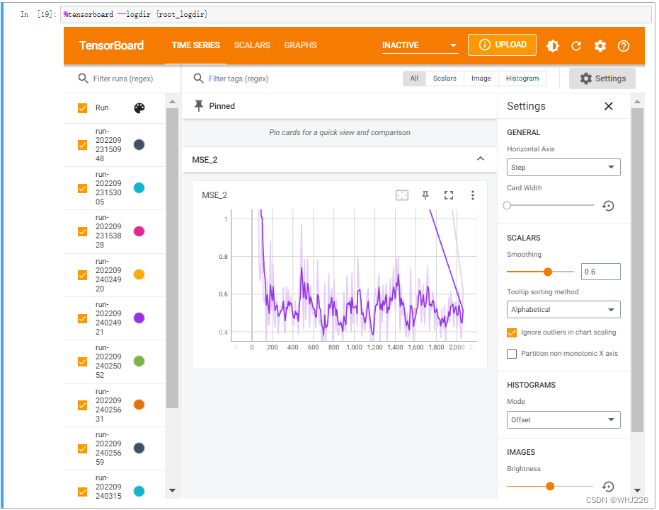
       [-0.8030471 ]], dtype=float32)

现在让我们看看TensorBoard。尝试转到SCALARS选项卡:

%tensorboard --logdir {root_logdir}

运行结果如下：

注意，它是交互式的一个界面，我们可以点击图片上的按钮来查看的。

下面是你可能会遇到的问题：

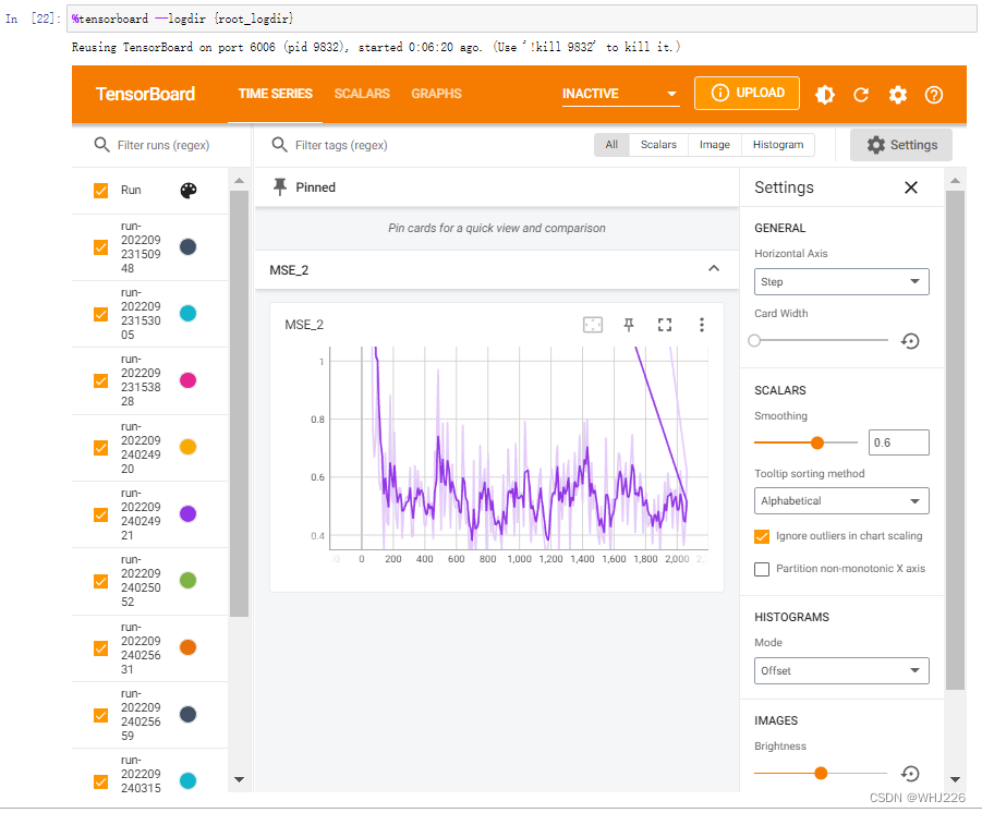
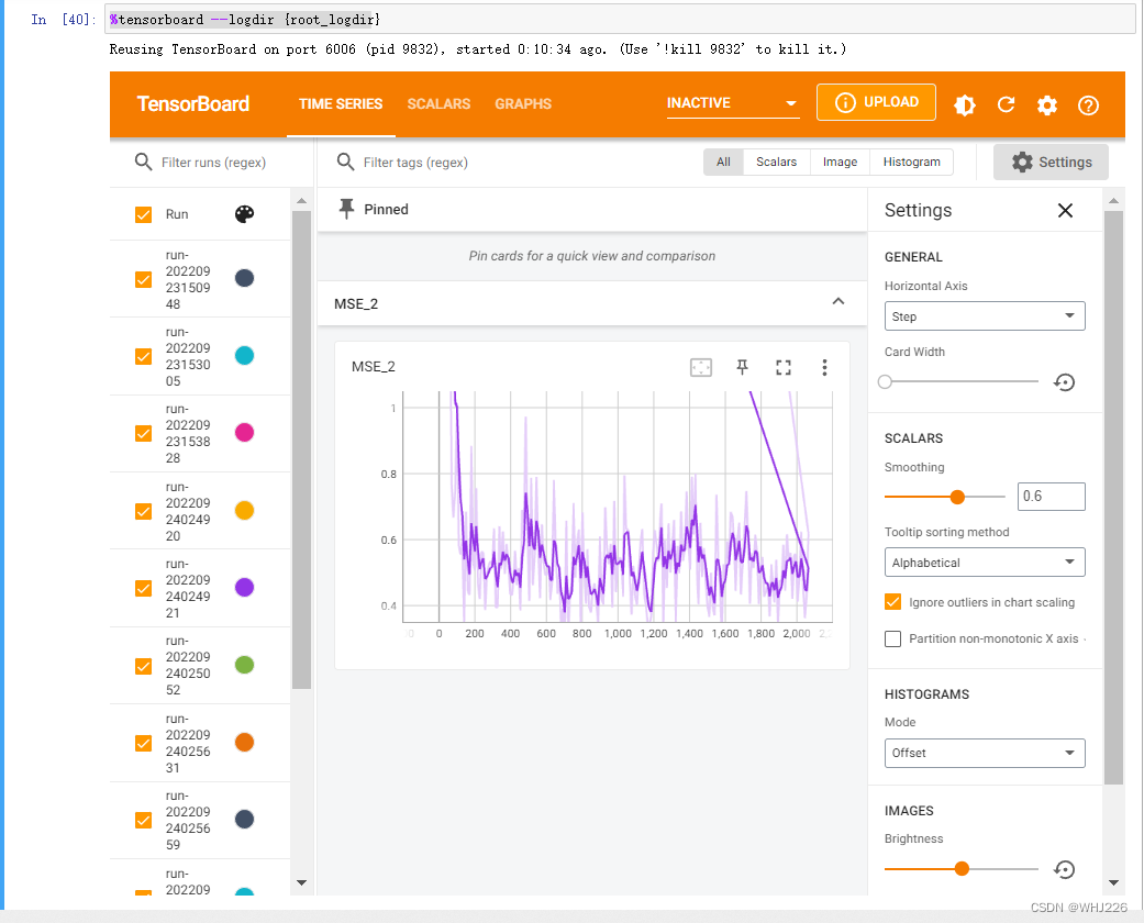
如果你再次（第二次）运行程序时，你可能会遇到“localhost已经拒绝了我们的连接请求”，只有第一次能运行显示正确的tensorboard可视界面，错误如下：

Reusing TensorBoard on port 6006 (pid 9832), started 0:10:34 ago. (Use '!kill 9832' to kill it.)

解决方法如下：

杀死进程（亲测可用）

首先打开cmd，输入下面这行代码：

taskkill /im tensorboard.exe /f

可能得到的反馈是：

成功: 已终止进程 "tensorboard.exe"，其 PID 为 12876。
成功: 已终止进程 "tensorboard.exe"，其 PID 为 9384。

或者?

错误: 没有找到进程 "tensorboard.exe"。

无妨，继续输入下面代码：

del /q %TMP%\.tensorboard-info\*

ok，返回jupyter运行程序即可。

参考：Reusing TensorBoard on port 6007 (pid 1320), started 0:01:15 ago. (Use ‘!kill 1320‘ to kill it.)_leo_liu-star的博客-CSDN博客

学习笔记——《机器学习实战：基于Scikit-Learn和TensorFlow》