文章目录
暂时浅过一遍,不求每个部分都理解很深度,后面通过复现项目来加深理解。
这里能理解个大概即可。
主要围绕这两个视频做一些笔记。
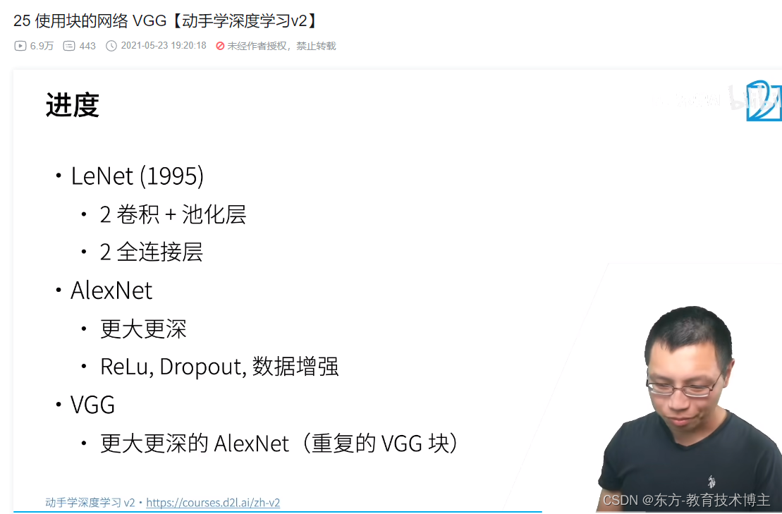
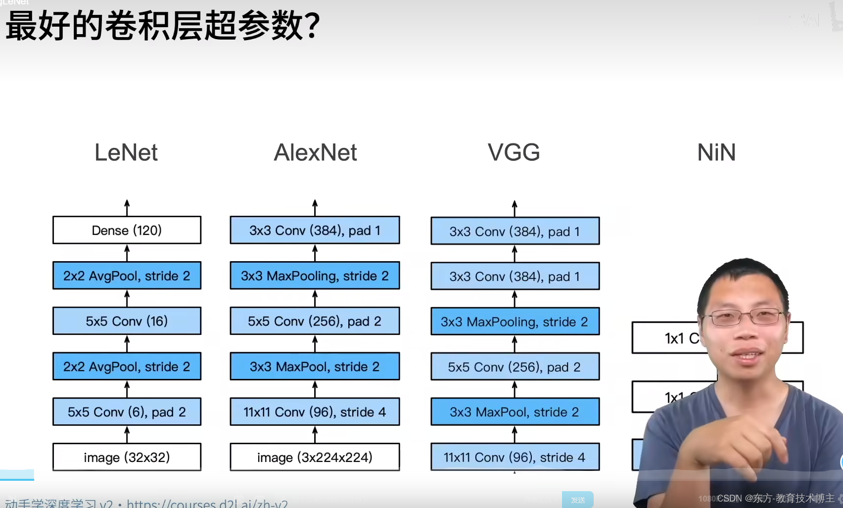
LeNet网络
代码:
# LeNet(LeNet-5) 由两个部分组成:卷积编码器和全连接层密集块
import torch
from torch import nn
from d2l import torch as d2l


class Reshape(torch.nn.Module):
    def forward(self, x):
        return x.view(-1, 1, 28, 28)  # 批量数自适应得到,通道数为1,图片为28X28


net = torch.nn.Sequential(
    Reshape(), nn.Conv2d(1, 6, kernel_size=5, padding=2), nn.Sigmoid(),
    nn.AvgPool2d(2, stride=2),
    nn.Conv2d(6, 16, kernel_size=5), nn.Sigmoid(),
    nn.AvgPool2d(kernel_size=2, stride=2), nn.Flatten(),
    nn.Linear(16 * 5 * 5, 120), nn.Sigmoid(),
    nn.Linear(120, 84), nn.Sigmoid(),
    nn.Linear(84, 10))

X = torch.rand(size=(1, 1, 28, 28), dtype=torch.float32)
for layer in net:
    X = layer(X)
    print(layer.__class__.__name__, 'output shape:\t', X.shape)  # 上一层的输出为这一层的输入
Reshape output shape:	 torch.Size([1, 1, 28, 28])
Conv2d output shape:	 torch.Size([1, 6, 28, 28])
Sigmoid output shape:	 torch.Size([1, 6, 28, 28])
AvgPool2d output shape:	 torch.Size([1, 6, 14, 14])
Conv2d output shape:	 torch.Size([1, 16, 10, 10])
Sigmoid output shape:	 torch.Size([1, 16, 10, 10])
AvgPool2d output shape:	 torch.Size([1, 16, 5, 5])
Flatten output shape:	 torch.Size([1, 400])
Linear output shape:	 torch.Size([1, 120])
Sigmoid output shape:	 torch.Size([1, 120])
Linear output shape:	 torch.Size([1, 84])
Sigmoid output shape:	 torch.Size([1, 84])
Linear output shape:	 torch.Size([1, 10])
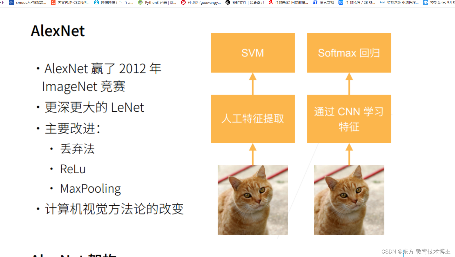
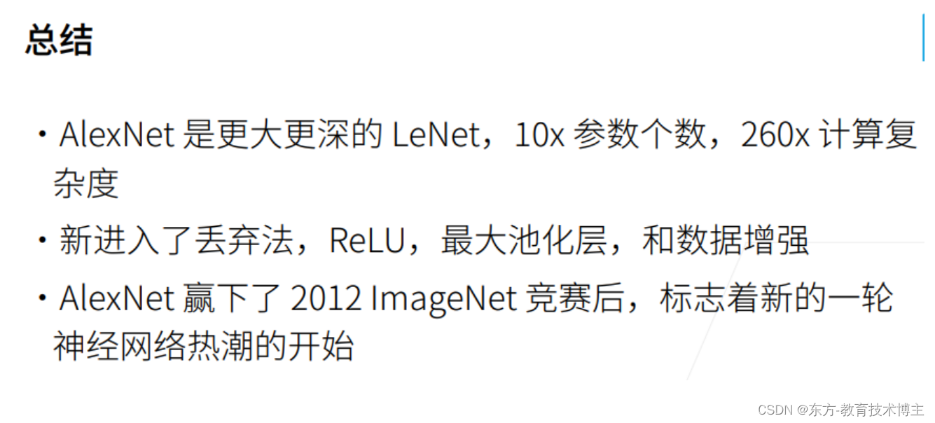
AlexNet
参考GitHub
因为我的方向是NLP,这里放代码,不多赘述
深度卷积神经网络 (AlexNet)
import torch
from torch import nn
from d2l import torch as d2l

net = nn.Sequential(
    nn.Conv2d(1,96,kernel_size=11,stride=4,padding=1),nn.ReLU(), # 数据集为fashion_mnist图片,所以输入通道为1,如果是Imagnet图片,则通道数应为3
    nn.MaxPool2d(kernel_size=3,stride=2),
    nn.Conv2d(96,256,kernel_size=5,padding=2),nn.ReLU(), # 256为输出通道数
    nn.MaxPool2d(kernel_size=3,stride=2),
    nn.Conv2d(256,384,kernel_size=3,padding=1),nn.ReLU(),
    nn.Conv2d(384,384,kernel_size=3,padding=1),nn.ReLU(),
    nn.Conv2d(384,256,kernel_size=3,padding=1),nn.ReLU(),
    nn.MaxPool2d(kernel_size=3,stride=2),nn.Flatten(),
    nn.Linear(6400,4096),nn.ReLU(),nn.Dropout(p=0.5),
    nn.Linear(4096,4096),nn.ReLU(),nn.Dropout(p=0.5),
    nn.Linear(4096,10))

X = torch.randn(1,1,224,224)
for layer in net:
    X = layer(X)
    print(layer.__class__.__name__,'Output shape:\t', X.shape)

# Fashion-MNIST图像的分辨率 低于ImageNet图像。将它们增加到224×224
batch_size = 128
train_iter, test_iter = d2l.load_data_fashion_mnist(batch_size,resize=224)

lr, num_epochs = 0.01, 10
d2l.train_ch6(net,train_iter,test_iter,num_epochs,lr,d2l.try_gpu())
结果:
Conv2d Output shape:	 torch.Size([1, 96, 54, 54])
ReLU Output shape:	 torch.Size([1, 96, 54, 54])
MaxPool2d Output shape:	 torch.Size([1, 96, 26, 26])
Conv2d Output shape:	 torch.Size([1, 256, 26, 26])
ReLU Output shape:	 torch.Size([1, 256, 26, 26])
MaxPool2d Output shape:	 torch.Size([1, 256, 12, 12])
Conv2d Output shape:	 torch.Size([1, 384, 12, 12])
ReLU Output shape:	 torch.Size([1, 384, 12, 12])
Conv2d Output shape:	 torch.Size([1, 384, 12, 12])
ReLU Output shape:	 torch.Size([1, 384, 12, 12])
Conv2d Output shape:	 torch.Size([1, 256, 12, 12])
ReLU Output shape:	 torch.Size([1, 256, 12, 12])
MaxPool2d Output shape:	 torch.Size([1, 256, 5, 5])
Flatten Output shape:	 torch.Size([1, 6400])
Linear Output shape:	 torch.Size([1, 4096])
ReLU Output shape:	 torch.Size([1, 4096])
Dropout Output shape:	 torch.Size([1, 4096])
Linear Output shape:	 torch.Size([1, 4096])
ReLU Output shape:	 torch.Size([1, 4096])
Dropout Output shape:	 torch.Size([1, 4096])
Linear Output shape:	 torch.Size([1, 10])
VGG
13年前辈,用可以重复的块(可以配置的)来构建deeplearning 模型
配置:可以选高配和低配。
这一思想深刻的影响到后面的模型。
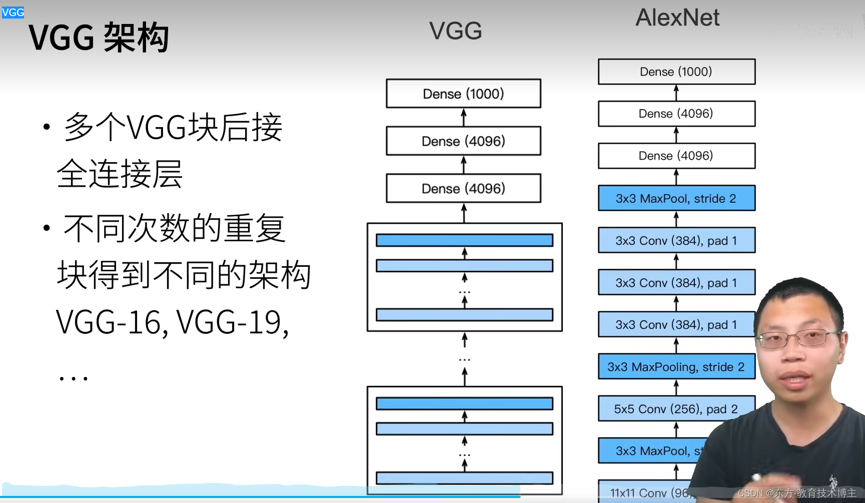
把AlexNet规则化了,
代码:
import torch
from torch import nn
from d2l import torch as d2l
def vgg_block(num_convs,in_channels,out_channels): # 卷积层个数、输入通道数、输出通道数
layers = []
for _ in range(num_convs):
layers.append(nn.Conv2d(in_channels,out_channels,kernel_size=3,padding=1))
layers.append(nn.ReLU())
in_channels = out_channels
layers.append(nn.MaxPool2d(kernel_size=2,stride=2))
return nn.Sequential(*layers) # *layers表示把列表里面的元素按顺序作为参数输入函数
conv_arch = ((1,64),(1,128),(2,256),(2,512),(2,512)) # 第一个参数为几层卷积,第二个参数为输出通道数
def vgg(conv_arch):
conv_blks = []
in_channels = 1
for (num_convs, out_channels) in conv_arch:
conv_blks.append(vgg_block(num_convs,in_channels,out_channels))
in_channels = out_channels
return nn.Sequential(*conv_blks, nn.Flatten(),
nn.Linear(out_channels * 7 * 7, 4096),nn.ReLU(),
nn.Dropout(0.5), nn.Linear(4096,4096),nn.ReLU(),
nn.Dropout(0.5), nn.Linear(4096,10))
net = vgg(conv_arch)
# 观察每个层输出的形状
X = torch.randn(size=(1,1,224,224))
for blk in net:
X = blk(X)
print(blk.__class__.__name__,'output shape:\t', X.shape) # VGG使得高宽减半,通道数加倍
# 由于VGG-11比AlexNet计算量更大,因此构建了一个通道数较少的网络
ratio = 4
small_conv_arch = [(pair[0], pair[1]//ratio) for pair in conv_arch] # 所有输出通道除以4
net = vgg(small_conv_arch)
lr, num_epochs, batch_size = 0.05, 10, 128
train_iter, test_iter = d2l.load_data_fashion_mnist(batch_size,resize=224)
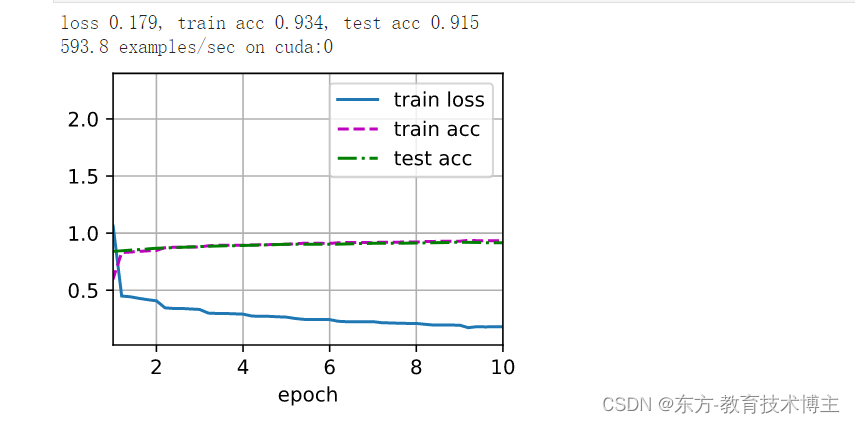
d2l.train_ch6(net,train_iter,test_iter,num_epochs,lr,d2l.try_gpu())
运行结果:
Sequential output shape:	 torch.Size([1, 64, 112, 112])
Sequential output shape:	 torch.Size([1, 128, 56, 56])
Sequential output shape:	 torch.Size([1, 256, 28, 28])
Sequential output shape:	 torch.Size([1, 512, 14, 14])
Sequential output shape:	 torch.Size([1, 512, 7, 7])
Flatten output shape:	 torch.Size([1, 25088])
Linear output shape:	 torch.Size([1, 4096])
ReLU output shape:	 torch.Size([1, 4096])
Dropout output shape:	 torch.Size([1, 4096])
Linear output shape:	 torch.Size([1, 4096])
ReLU output shape:	 torch.Size([1, 4096])
Dropout output shape:	 torch.Size([1, 4096])
Linear output shape:	 torch.Size([1, 10])
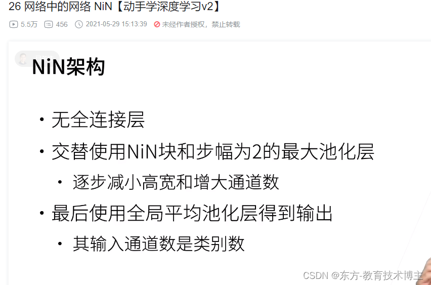
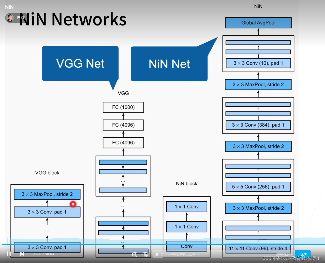
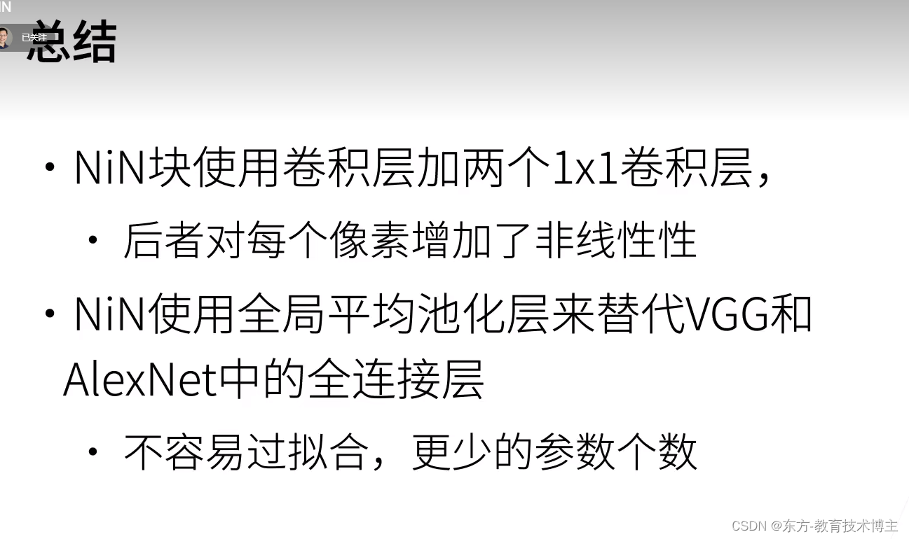
NIN(网络中的概念)
用到的不多,但是提出了很多关键性的概念,后面都会用到
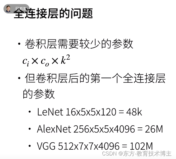
问题背景:
卷积层之后的第一个全连接层会带来大量的内存开销和计算量。且很容易过拟合。
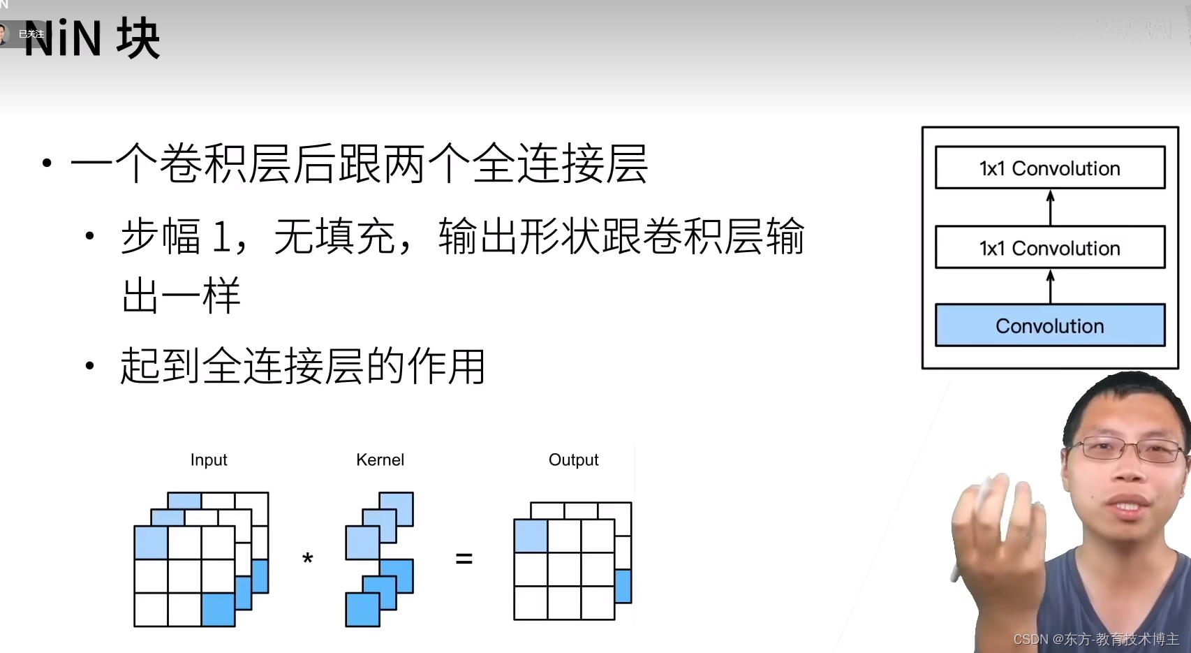
作用是为了混合通道数。
实现代码:
import torch
from torch import nn
from d2l import torch as d2l
def nin_block(in_channels, out_channels, kernel_size, strides, padding):
return nn.Sequential(nn.Conv2d(in_channels, out_channels, kernel_size, strides,padding),
nn.ReLU(), nn.Conv2d(out_channels, out_channels, kernel_size=1),
nn.ReLU(), nn.Conv2d(out_channels, out_channels, kernel_size=1),
nn.ReLU())
net = nn.Sequential(nin_block(1,96,kernel_size=11,strides=4,padding=0),
nn.MaxPool2d(3,stride=2),
nin_block(96,256,kernel_size=5,strides=1,padding=2),
nn.MaxPool2d(3,stride=2),
nin_block(256,384,kernel_size=3,strides=1,padding=1),
nn.MaxPool2d(3,stride=2),nn.Dropout(0.5),
nin_block(384,10,kernel_size=3,strides=1,padding=1),
nn.AdaptiveAvgPool2d((1,1)),
nn.Flatten())
# 查看每个块的输出形状
X = torch.rand(size=(1,1,224,224))
for layer in net:
X = layer(X)
print(layer.__class__.__name__, 'output shape:\t', X.shape)
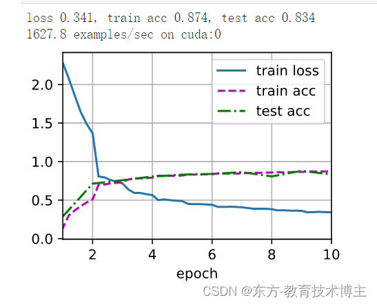
# 训练模型
lr, num_epochs, batch_size = 0.1, 10, 128
train_iter, test_iter = d2l.load_data_fashion_mnist(batch_size, resize=224)
d2l.train_ch6(net, train_iter, test_iter, num_epochs, lr, d2l.try_gpu())
结果:
Sequential output shape:	 torch.Size([1, 96, 54, 54])
MaxPool2d output shape:	 torch.Size([1, 96, 26, 26])
Sequential output shape:	 torch.Size([1, 256, 26, 26])
MaxPool2d output shape:	 torch.Size([1, 256, 12, 12])
Sequential output shape:	 torch.Size([1, 384, 12, 12])
MaxPool2d output shape:	 torch.Size([1, 384, 5, 5])
Dropout output shape:	 torch.Size([1, 384, 5, 5])
Sequential output shape:	 torch.Size([1, 10, 5, 5])
AdaptiveAvgPool2d output shape:	 torch.Size([1, 10, 1, 1])
Flatten output shape:	 torch.Size([1, 10])
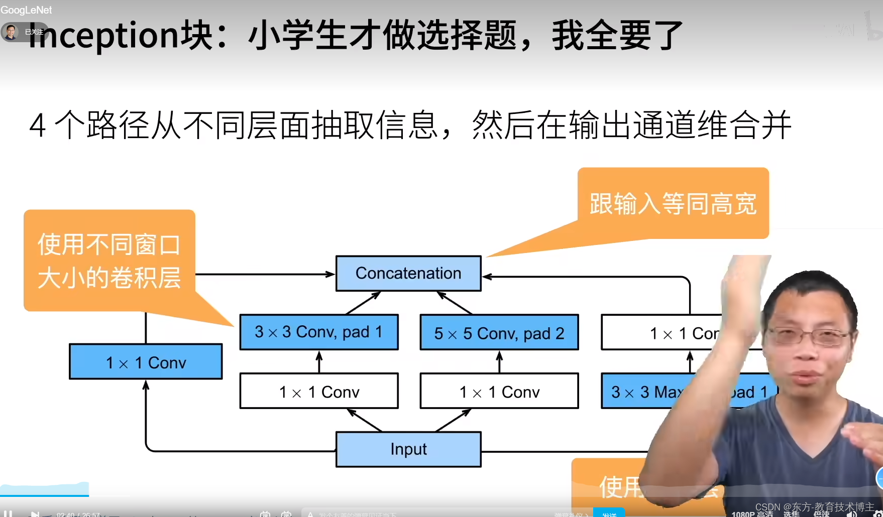
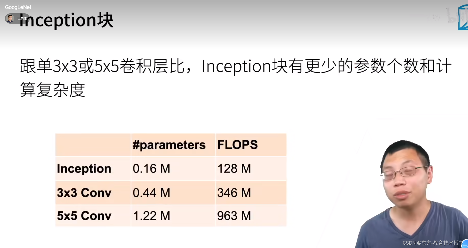
含并行连接的网络GoogLeNet / Inception V3
一篇不错的笔记
现在比较用的多:
第一个卷积层个数超过100的,和LeNet无关系(致敬+玩个梗)

但是看B站评论区。。。

通过并行通道达到上百个卷积
(平行加起来可以达到上百层)
通道数(可能是遍历之后机器选的最优解),所以说比较奇怪。
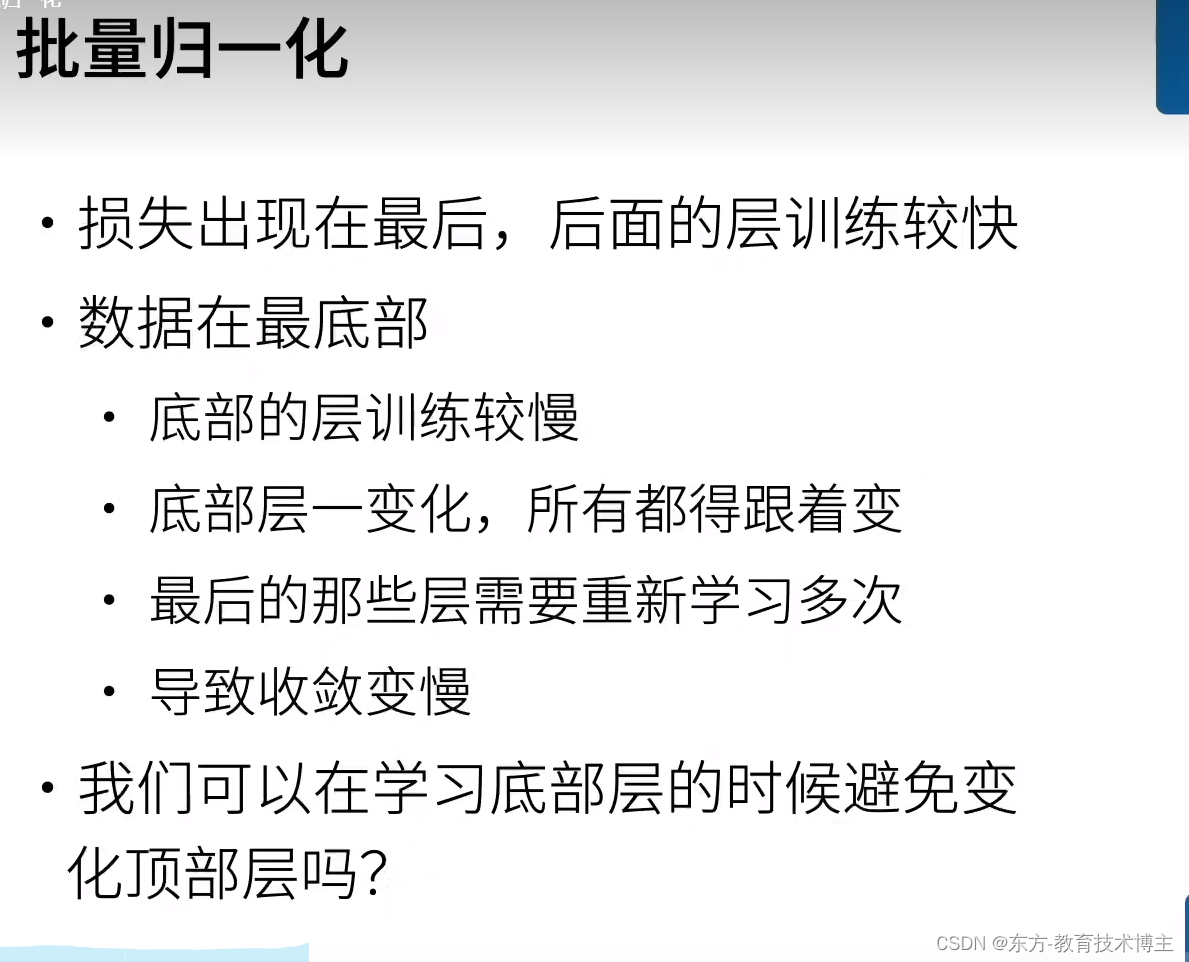
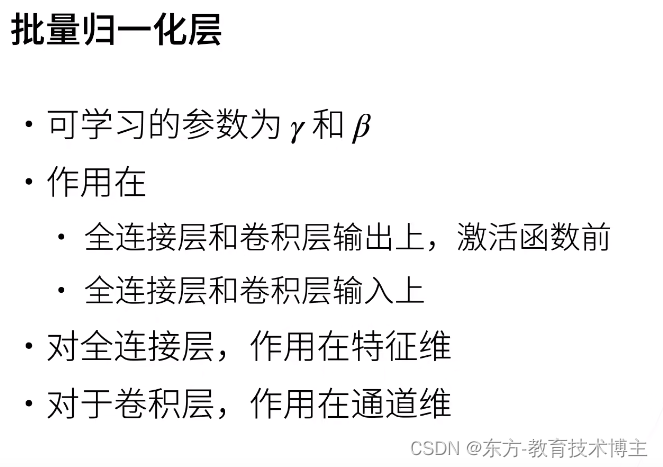
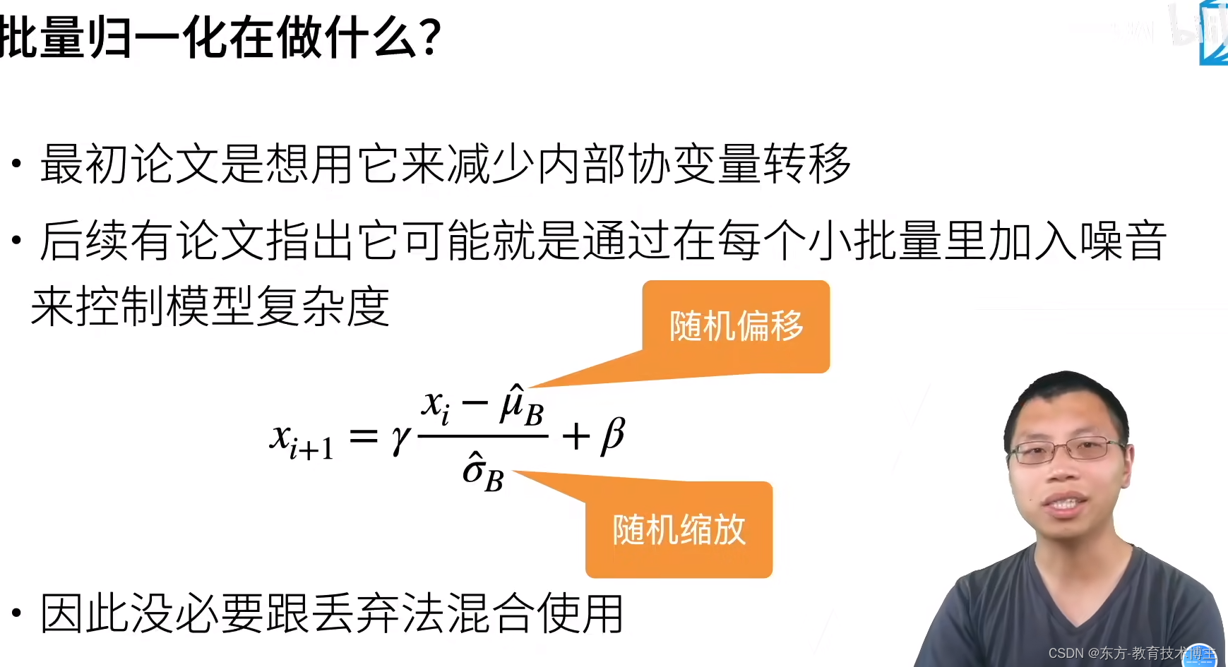
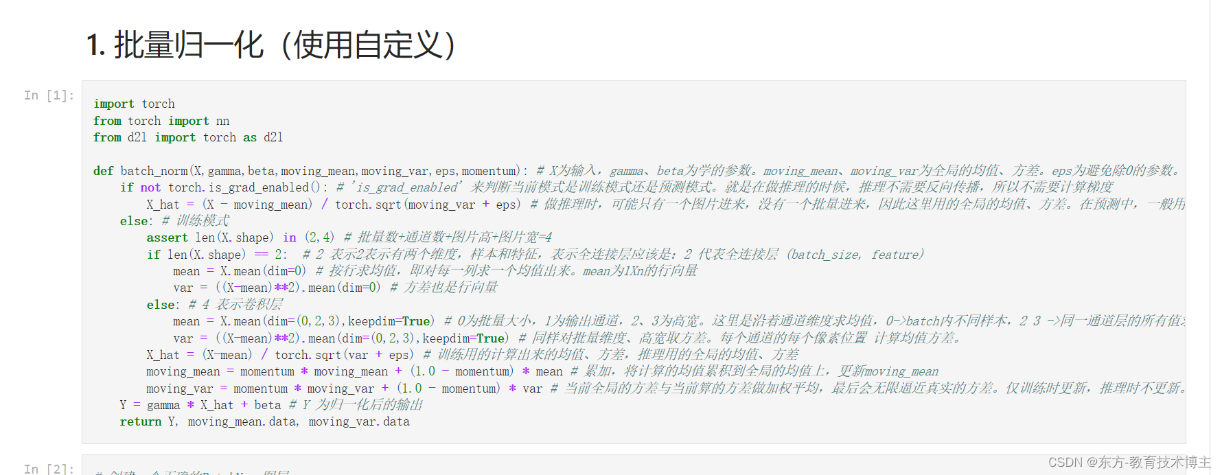
批量 归一化
B站一篇不错的笔记
其实这个大佬。。。。写的很多笔记都不错哈哈去和他要好友位了。
现在的卷积神经网络或多或少都用到了这一个层。
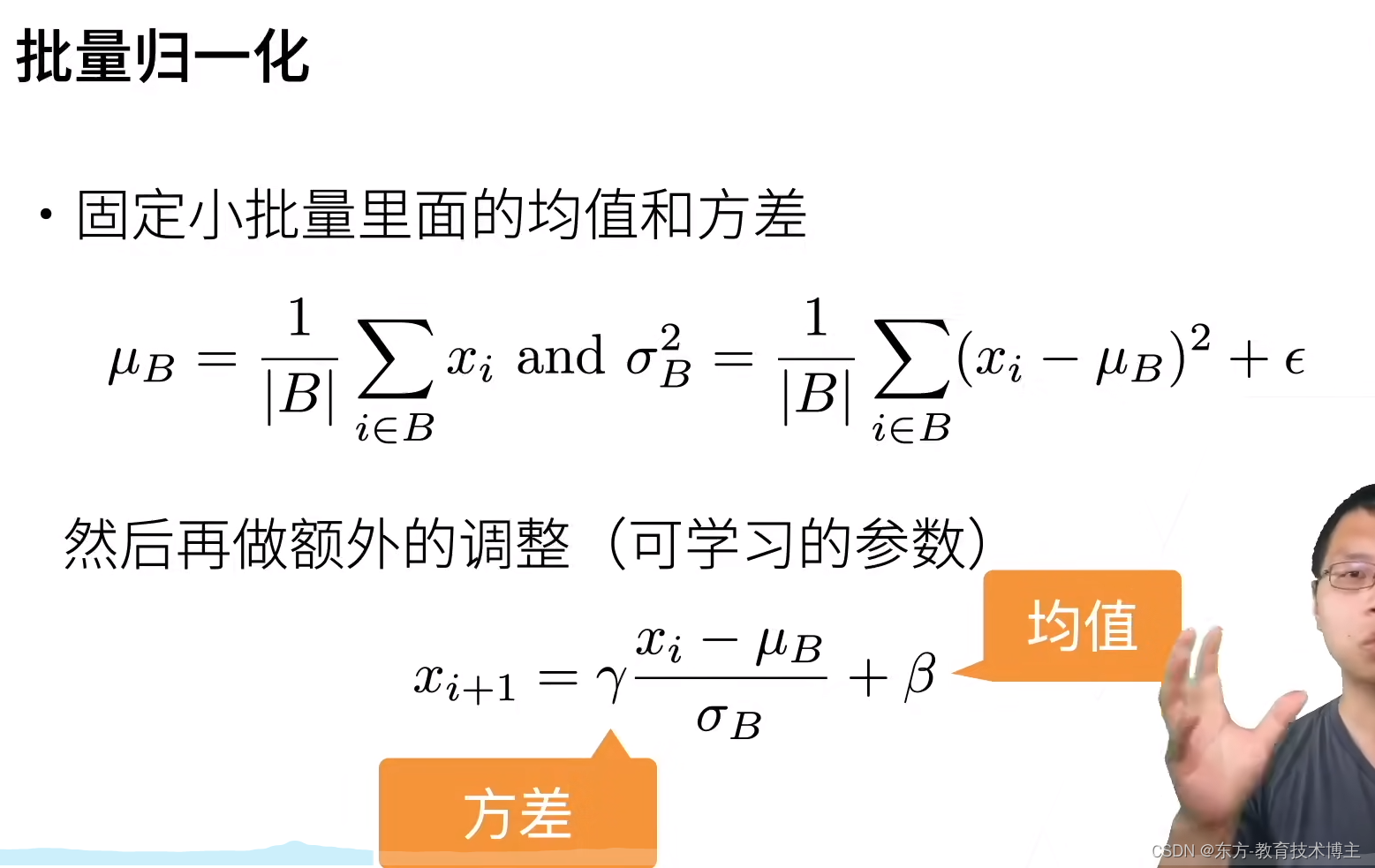

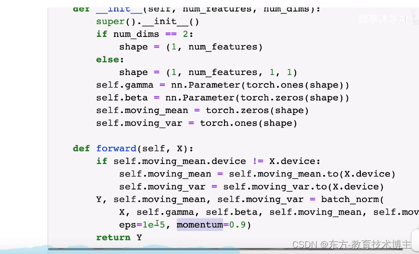
注意事项:这个eps会根据模型具体情况确定,moment一般是0.9
具体应用:
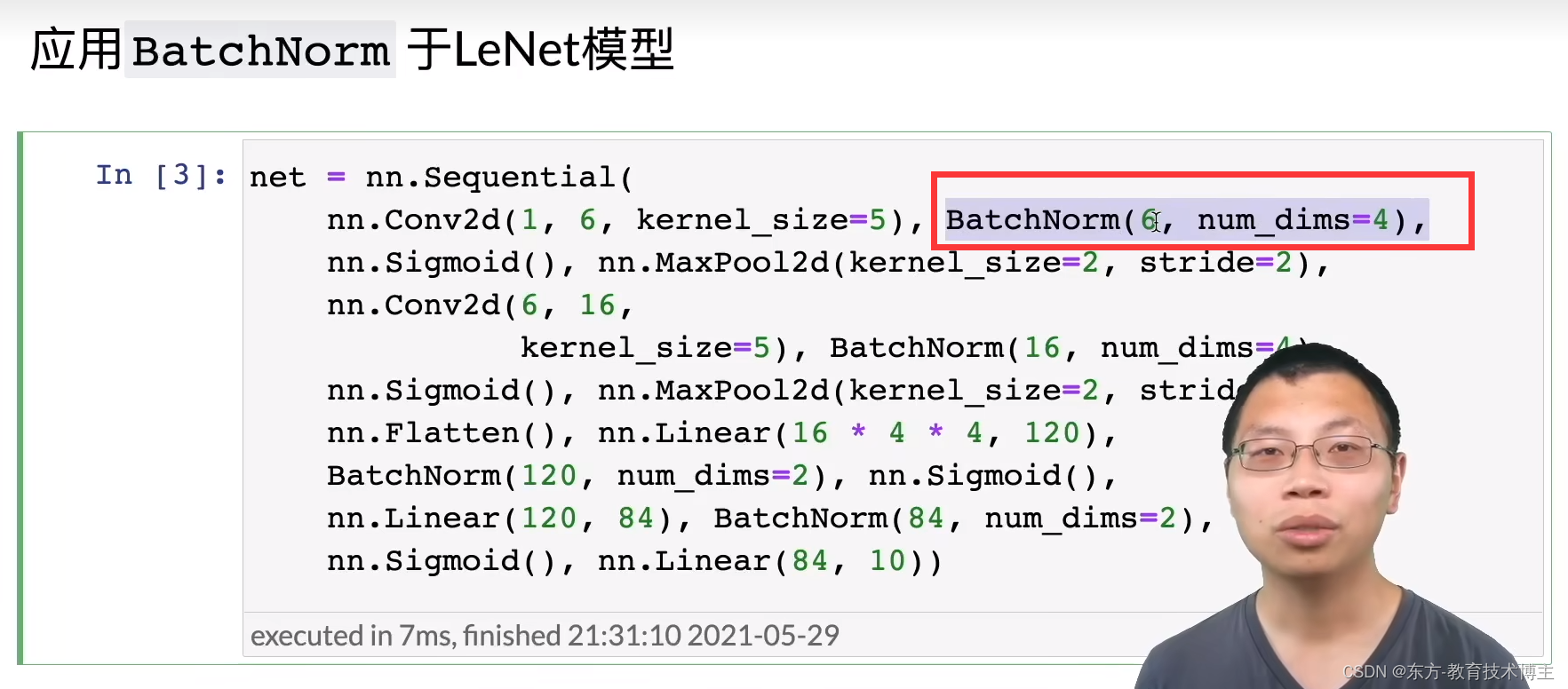
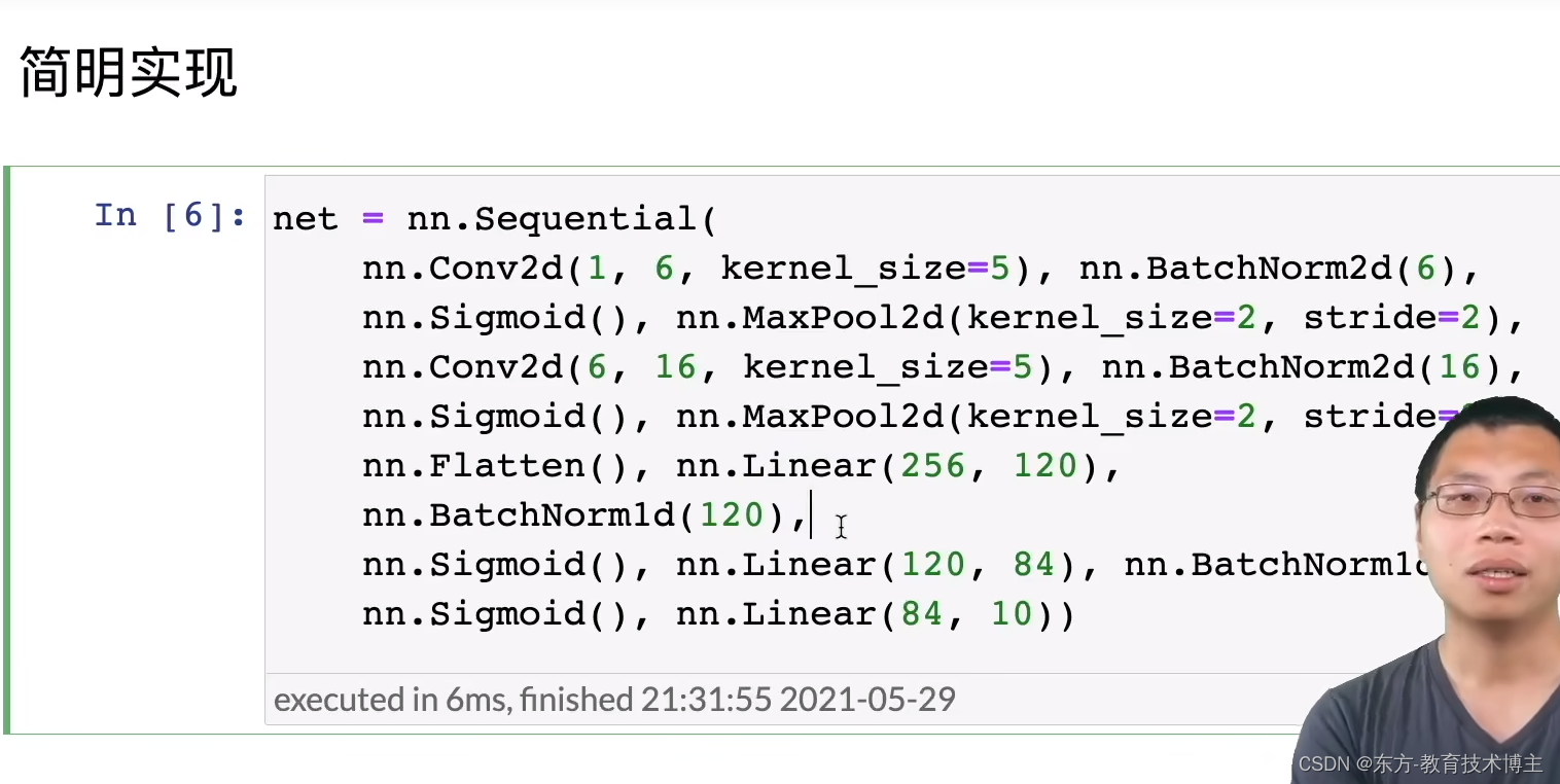
pytorch会自动加合适的维度,但是有时候加的不一定很好。
一些B站评论区大佬讨论


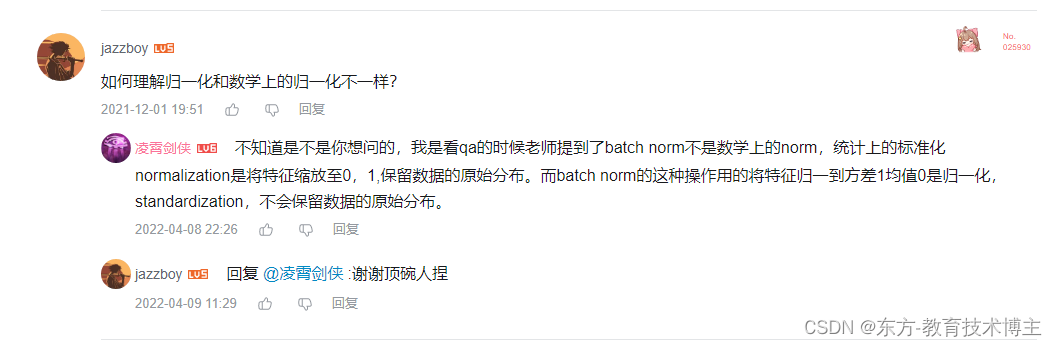
放个链接,不再讲解了。
再次感谢
残差网络ResNet
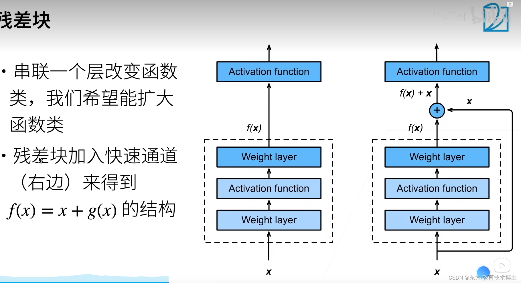

ResNet为什么能训练一千层
关键在于怎样处理梯度消失的。
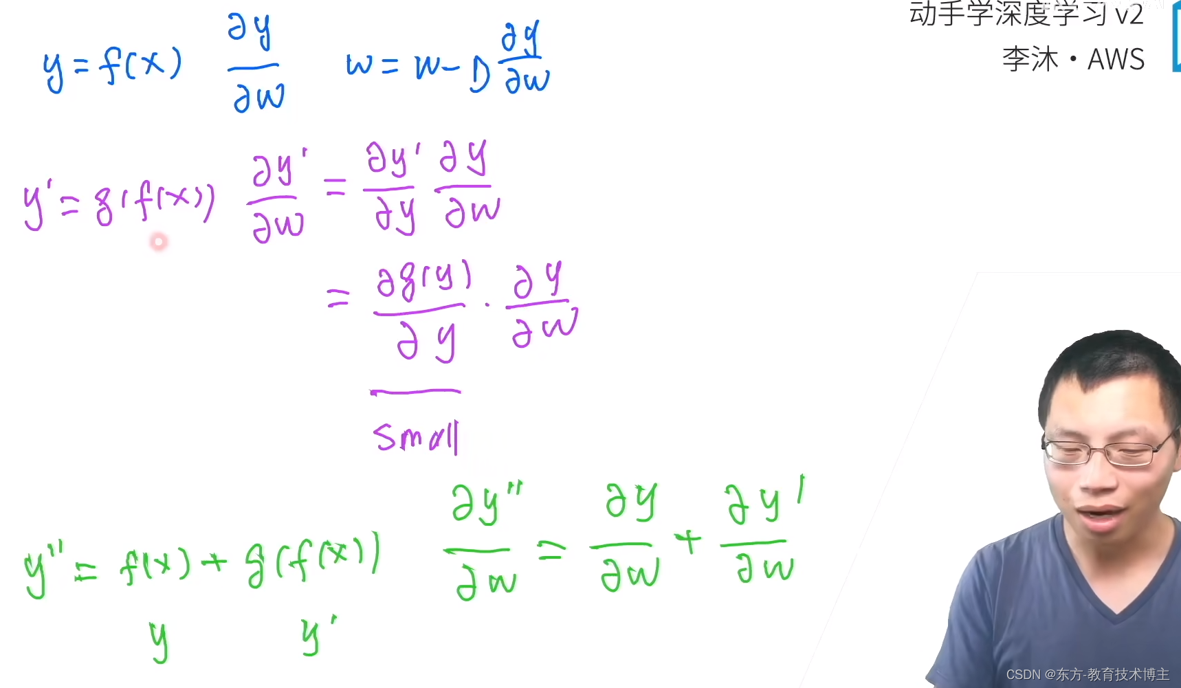
下面这个公式