目录
5.1 卷积
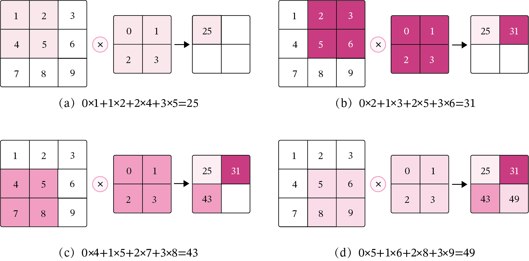
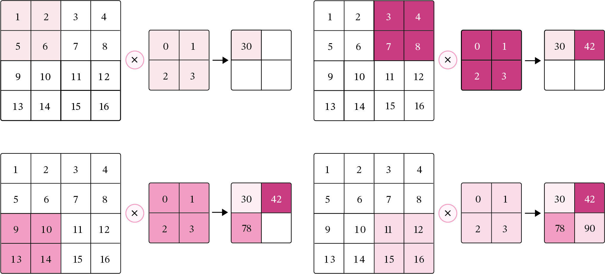
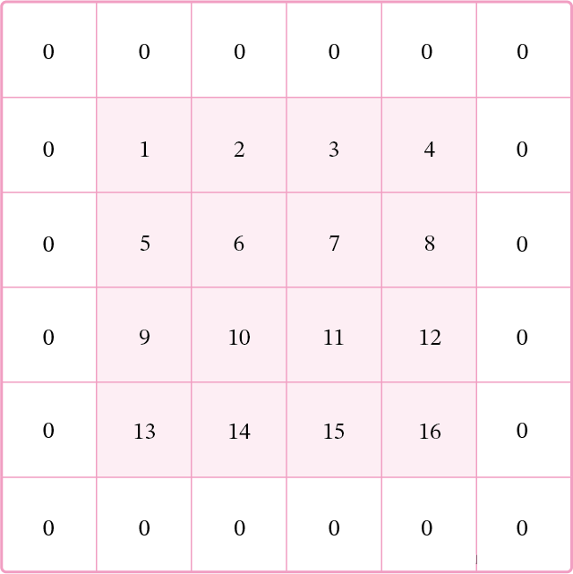
5.1.2 二维卷积算子
在本书后面的实现中,算子都继承paddle.nn.Layer飞桨API进行实现,这样我们就可以不用手工写backword()的代码实现。
import torch
import torch.nn as nn

class Conv2D(nn.Module):
    def __init__(self, kernel_size,
                    weight_attr=torch.tensor([[0., 1.],[2., 3.]])):
        super(Conv2D, self).__init__()
        # 使用'paddle.create_parameter'创建卷积核
        # 使用'paddle.ParamAttr'进行参数初始化
        self.weight = nn.Parameter(weight_attr)
    def forward(self, X):
        """
        输入:
            - X:输入矩阵,shape=[B, M, N],B为样本数量
        输出:
            - output:输出矩阵
        """
        u, v = self.weight.shape
        output = torch.zeros([X.shape[0], X.shape[1] - u + 1, X.shape[2] - v + 1])
        for i in range(output.shape[1]):
            for j in range(output.shape[2]):
                output[:, i, j] = torch.sum(X[:, i:i+u, j:j+v]*self.weight, axis=[1,2])
        return output

# 随机构造一个二维输入矩阵
torch.seed()
inputs = torch.tensor([[[1.,2.,3.],[4.,5.,6.],[7.,8.,9.]]])

conv2d = Conv2D(kernel_size=2)
outputs = conv2d(inputs)
print("input: {}, \noutput: {}".format(inputs, outputs))
torch.Size([2, 2])
input: tensor([[[1., 2., 3.],
         [4., 5., 6.],
         [7., 8., 9.]]]),
output: tensor([[[25., 31.],
         [43., 49.]]], grad_fn=<CopySlices>)
5.1.3 二维卷积的参数量和计算量
随着隐藏层神经元数量的变多以及层数的加深,
使用全连接前馈网络处理图像数据时,参数量会急剧增加。
如果使用卷积进行图像处理,相较于全连接前馈网络,参数量少了非常多。
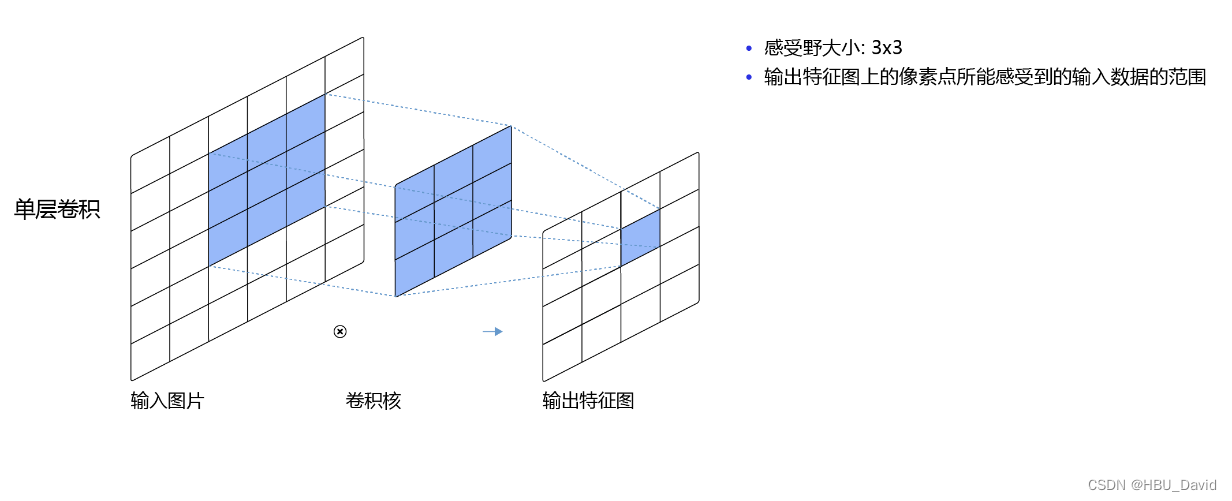
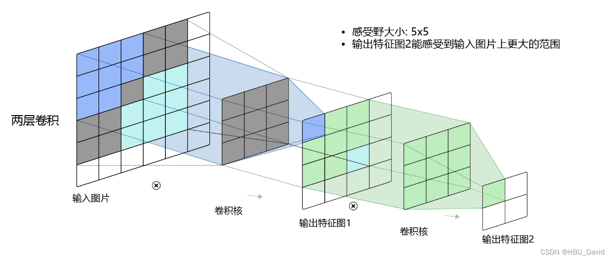
5.1.4 感受野
5.1.5 卷积的变种
5.1.5.1 步长(Stride)
5.1.5.2 零填充(Zero Padding)
5.1.6 带步长和零填充的二维卷积算子
从输出结果看出,使用3×3大小卷积,
padding为1,
当stride=1时,模型的输出特征图与输入特征图保持一致;
当stride=2时,模型的输出特征图的宽和高都缩小一倍。
【使用pytorch实现】
class Conv2D(nn.Module):
    def __init__(self, kernel_size,stride=1, padding=0,
                    weight_attr=torch.tensor([[0., 1.],[2., 3.]])):
        super(Conv2D, self).__init__()
        # 使用'paddle.create_parameter'创建卷积核
        # 使用'paddle.ParamAttr'进行参数初始化
        self.weight = nn.Parameter(weight_attr)
        # 步长
        self.stride = stride
        # 零填充
        self.padding = padding

    def forward(self, X):
        """
        输入:
            - X:输入矩阵,shape=[B, M, N],B为样本数量
        输出:
            - output:输出矩阵
        """
        u, v = self.weight.shape
        output = torch.zeros([X.shape[0], X.shape[1] - u + 1, X.shape[2] - v + 1])
        for i in range(output.shape[1]):
            for j in range(output.shape[2]):
                output[:, i, j] = torch.sum(X[:, i:i+u, j:j+v]*self.weight, axis=[1,2])
        return output

# 随机构造一个二维输入矩阵
torch.seed()
inputs = torch.tensor([[[1.,2.,3.],[4.,5.,6.],[7.,8.,9.]]])

conv2d = Conv2D(kernel_size=2)
outputs = conv2d(inputs)
print("input: {}, \noutput: {}".format(inputs, outputs))

inputs = torch.randn(size=[2, 8, 8])
conv2d_padding = Conv2D(kernel_size=3, padding=1)
outputs = conv2d_padding(inputs)
print("When kernel_size=3, padding=1 stride=1, input's shape: {}, output's shape: {}".format(inputs.shape, outputs.shape))
conv2d_stride = Conv2D(kernel_size=3, stride=2, padding=1)
outputs = conv2d_stride(inputs)
print("When kernel_size=3, padding=1 stride=2, input's shape: {}, output's shape: {}".format(inputs.shape, outputs.shape))
When kernel_size=3, padding=1 stride=1, input's shape: torch.Size([2, 8, 8]), output's shape: torch.Size([2, 8, 8])
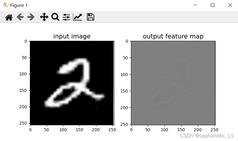
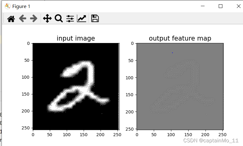
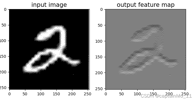
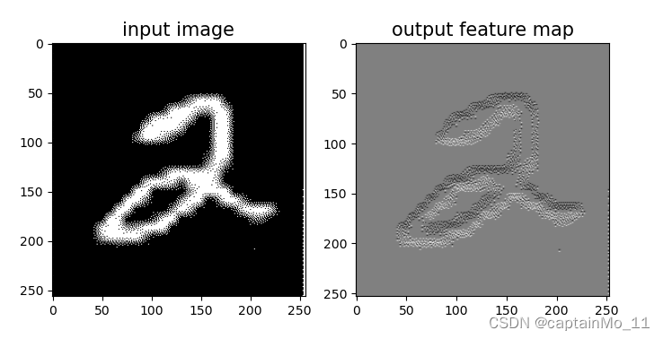
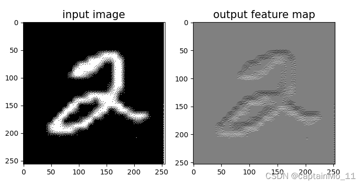
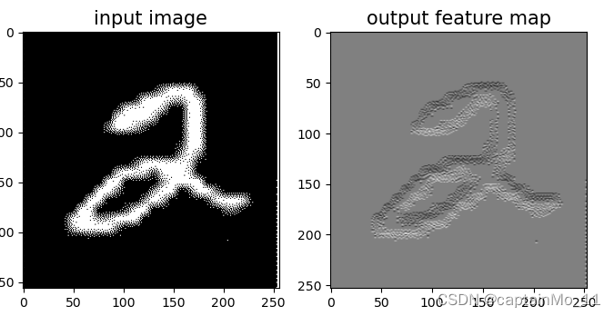
When kernel_size=3, padding=1 stride=2, input's shape: torch.Size([2, 8, 8]), output's shape: torch.Size([2, 4, 4])5.1.7 使用卷积运算完成图像边缘检测任务
【使用pytorch实现】
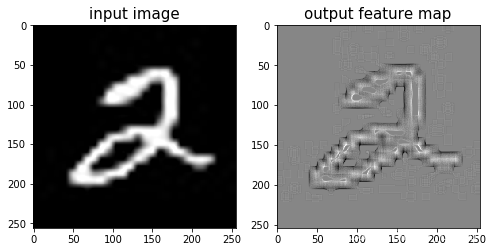
# 可视化结果
plt.figure(figsize=(8, 4))
f = plt.subplot(121)
f.set_title('input image', fontsize=15)
plt.imshow(img)
f = plt.subplot(122)
f.set_title('output feature map', fontsize=15)
plt.imshow(outputs.detach().squeeze(), cmap='gray')
plt.savefig('conv-vis.pdf')
plt.show()
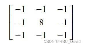
选做
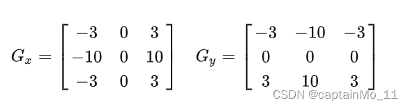
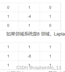
实现一些传统边缘检测算子,如:Roberts、Prewitt、Sobel、Scharr、Kirsch、Robinson、Laplacian
Roberts:
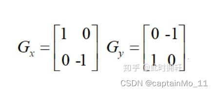
?Prewitt:
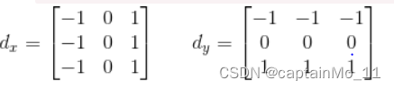
?
?Sobel:
?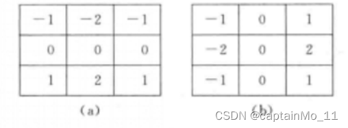
?
?Scharr:
?Kirsch:
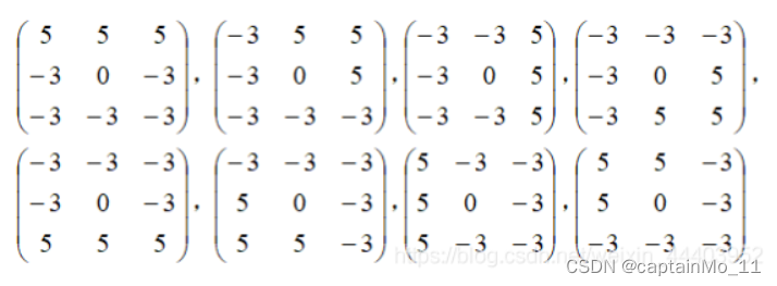
?
?Robinson:
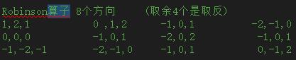
?
?Laplacian
?
总结:了解卷积的基本流程,了解卷积核的设置,步长的的设置,是否需要填充等问题