note
- KGAT���KG��GAT,��֪ʶͼ����Ԫ�������,����GAT������Ϣ����,�ۺϳ���Ʒ���������û��������м���õ�Ԥ��ֵ����ʵ�����KG,�������Ŷ�֮ǰҲֱ��ʹ��GNN����NGCF��LightGCN��
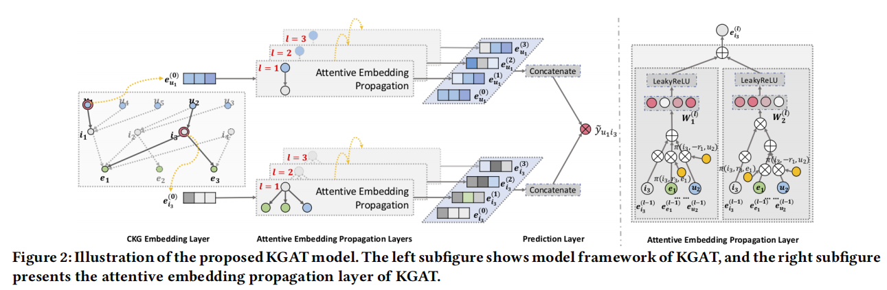
- KGAT������CKGǶ���ʾ��ʹ��TransRģ�ͻ��ʵ���ϵ��embedding;Ȼ����attention��ʾ������,ʹ��attention���ÿ���ھӽڵ�Ĺ���Ȩ��,��Ҫ��ʵ��ڵ� h h h������Ƕ���ʾ e h e_h eh?�������������Ƕ���ʾ e N h \boldsymbol{e}_{\mathcal{N}_h} eNh??�ں�����,�õ��ڵ� h h h���±�ʾ e h ( 1 ) \boldsymbol{e}_h^{(1)} eh(1)?,������ںϷ���Ҳ������;����Ԥ������������û���������Ʒ�����ĵ�����,����ʵlabel���н�������ʧ��������loss,�Ż�Ȩ�ء�
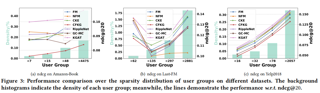
- KGAT�ɻ���High-Order Connectivity���б���ѧϰ����������������ʵ��,KGATЧ������CKE��RippleNet��ģ�͡�
����Ŀ¼
�㡢KGAT����
���ĵ�ַ:https://arxiv.org/pdf/1905.07854.pdf
���Ĵ���:https://github.com/xiangwang1223/knowledge_graph_attention_network
һ�����Ķ���
1.1 motivation
��ͳ���мලѧϰ������,�������ӷֽ��,�ڳ�ȡ������������������,��ÿ����������һ���������¼���Ԥ��,������������֮�����ڵĹ�ϵ��֪ʶͼ��������֮��ͨ�����Թ�������,ʹ������֮�䲻�ٶ���Ԥ�⡣KGAT��������������ʵ��,����Neural FM��RippleNet�ȡ�
KGAT���û�-��Ʒ�Ľ�������ͼ��֪ʶͼ���ں���һ�𡪡�Э֪ͬʶͼCKG,����ͼ��ϵ���û�user��item�Ķ�������ͼ�ںϵ�һ��ͼ�ռ�,���ں�CF��Ϣ��KG��Ϣ,KKGҲ�ܷ��ָ��߽Ĺ�ϵ��Ϣ����Э֪ͬʶͼ G \mathcal{G} G��:
- �ڵ����ʵ�塢�û�����Ʒ;
- ��ϵ����ԭ��֪ʶͼ�Ĺ�ϵ���һ����Ӧ�û�-��Ʒ�Ľ�����ϵ��
1.2 ͼ�����ͻ�ȡ�ڽӱ�
����ھӵĽڵ�embedding��ϵembedding,ʹ��get_neighbors����,ͨ����Ʒid�õ����ھӼ��������ǵĹ�ϵ��id,Ȼ��ͨ���ھӺ�ϵid�õ��ھ�ʵ�����ϵ��embedding�ķ���,���м��adj_entity��adj_Relation�ֱ���ͼ������õ���ָ���������ڽ��б���
# �õ��ھӵĽڵ�embedding��ϵembedding
def get_neighbors( self, items ):
e_ids = [self.adj_entity[ item ] for item in items ]
r_ids = [ self.adj_relation[ item ] for item in items ]
e_ids = torch.LongTensor( e_ids )
r_ids = torch.LongTensor( r_ids )
neighbor_entities_embs = self.entity_embs( e_ids )
neighbor_relations_embs = self.relation_embs( r_ids )
return neighbor_entities_embs, neighbor_relations_embs
adj_entity��adj_Relation�������е�dataloader4KGNN.construct_adj��������ֵ(ͨ��kg�ڽ��б��õ�ʵ���ڽ��б���ϵ�ڽ��б�),��������Ϣ����ʱ��Ҫͨ�����ڽӾ���,��õ�ǰ�ڵ���ھӽڵ�embedding��ϵembedding��
# ����kg�ڽ��б�,�õ�ʵ���ڽ��б���ϵ�ڽ��б�
def construct_adj( neighbor_sample_size, kg_indexes, entity_num ):
print('����ʵ���ڽ��б���ϵ�ڽ��б�')
adj_entity = np.zeros([ entity_num, neighbor_sample_size ], dtype = np.int64 )
adj_relation = np.zeros([ entity_num, neighbor_sample_size ], dtype = np.int64 )
for entity in range( entity_num ):
neighbors = kg_indexes[ str( entity ) ]
n_neighbors = len( neighbors )
if n_neighbors >= neighbor_sample_size:
sampled_indices = np.random.choice( list( range( n_neighbors ) ),
size = neighbor_sample_size, replace = False )
else:
sampled_indices = np.random.choice( list( range( n_neighbors ) ),
size = neighbor_sample_size, replace = True )
adj_entity[ entity ] = np.array( [ neighbors[i][0] for i in sampled_indices ] )
adj_relation[ entity] = np.array( [ neighbors[i][1] for i in sampled_indices ] )
return adj_entity, adj_relation
1.3 �ع���ǰ��GAT����
�����GAT����Ϊ�˼����ʹ��dgl�����dglnn.GATConv��,�����������Ľڵ���������ͼע��������(GAT)��Դ������ Graph Attention Networks������ѧ����Ϊ,
x
i
��
=
��
i
,
i
��
x
i
+
��
j
��
N
(
i
)
��
i
,
j
��
x
j
,
\mathbf{x}^{\prime}_i = \alpha_{i,i}\mathbf{\Theta}\mathbf{x}_{i} + \sum_{j \in \mathcal{N}(i)} \alpha_{i,j}\mathbf{\Theta}\mathbf{x}_{j},
xi��?=��i,i?��xi?+j��N(i)��?��i,j?��xj?,
GAT�����е�attention mechanismһ��,GAT�ļ���Ҳ��Ϊ������:
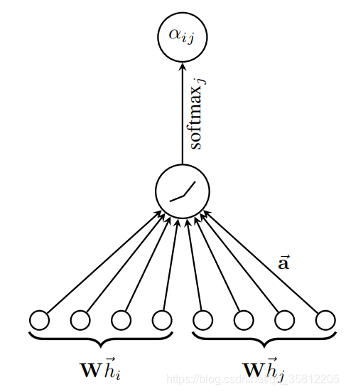
(1)����ע����ϵ��(attention coefficient):(��ͼ���ԡ�GRAPH ATTENTION NETWORKS��)������ע����ϵ��
��
i
,
j
\alpha_{i,j}
��i,j?�ļ��㷽��Ϊ,
��
i
,
j
=
exp
?
(
L
e
a
k
y
R
e
L
U
(
a
?
[
��
x
i
?
��
?
��
x
j
]
)
)
��
k
��
N
(
i
)
��
{
i
}
exp
?
(
L
e
a
k
y
R
e
L
U
(
a
?
[
��
x
i
?
��
?
��
x
k
]
)
)
.
\alpha_{i,j} = \frac{ \exp\left(\mathrm{LeakyReLU}\left(\mathbf{a}^{\top} [\mathbf{\Theta}\mathbf{x}_i \, \Vert \, \mathbf{\Theta}\mathbf{x}_j] \right)\right)} {\sum_{k \in \mathcal{N}(i) \cup \{ i \}} \exp\left(\mathrm{LeakyReLU}\left(\mathbf{a}^{\top} [\mathbf{\Theta}\mathbf{x}_i \, \Vert \, \mathbf{\Theta}\mathbf{x}_k] \right)\right)}.
��i,j?=��k��N(i)��{i}?exp(LeakyReLU(a?[��xi?����xk?]))exp(LeakyReLU(a?[��xi?����xj?]))?.
(2)��Ȩ���(aggregate):����(1)��ϵ��,��������Ȩ���(aggregate)

class GAT(nn.Module):
    def __init__(self,in_size, hid_size, out_size, heads):
        super().__init__()
        self.gat_layers = nn.ModuleList()
        # two-layer GAT(attention)
        self.gat_layers.append(dglnn.GATConv(in_size, hid_size, heads[0], feat_drop=0.6, attn_drop=0.6, activation=F.elu))
        # GATConv: in_feat, out_feat, num_head(multi-head)
        self.gat_layers.append(dglnn.GATConv(hid_size*heads[0], out_size, heads[1], feat_drop=0.6, attn_drop=0.6, activation=None))

    def forward(self, g, inputs):
        h = inputs
        for i, layer in enumerate(self.gat_layers):
            h = layer(g, h)
            if i == 1:  # last layer
                h = h.mean(1)
            else:       # other layer(s)
                h = h.flatten(1)
        return h
ʹ�ý�������ʧ����,��dgl������ʹ��train_mask��ʾ����ѵ�����Ľڵ�,�����Ӧλ�õ�train_maskΪfalse���ʾ����ýڵ㲻�������ѵ������
����KGATģ��
2.1 CKGǶ���ʾ��
�ò�Ϊ�˵õ�֪ʶͼ�ṹ��ʵ���ϵ��Ƕ���ʾ,ʹ��TransRģ��,TransRģ��ʹ����Ԫ��(h, r, t)�ڹ�ϵr��ͶӰƽ������ƽ�ƹ�ϵ:
g
(
h
,
r
1
,
t
)
=
��
W
r
e
h
+
e
r
?
W
r
e
t
��
2
2
g\left(h, r_1, t\right)=\left\|\boldsymbol{W}_r \boldsymbol{e}_h+\boldsymbol{e}_{\mathrm{r}}-\boldsymbol{W}_r \boldsymbol{e}_t\right\|_2^2
g(h,r1?,t)=��Wr?eh?+er??Wr?et?��22?����:
- W r �� R k �� d \boldsymbol{W}_r \in \mathbb{R}^{k \times d} Wr?��Rk��d �ǹ�ϵ r r r �ı任����,��ʵ���dάʵ��ռ�ͶӰ��kά��ϵ�ռ���;
- g ( h , r , t ) g(h, r, t) g(h,r,t) ����ԽС, ��ʾ��Ԫ�� ( h , r , t ) (h, r, t) (h,r,t) �����ĸ���Խ��,����Ԫ��Խ���š�
ʹ��pairwise ranking loss��Ϊѵ����ʧ����:
L
K
G
=
��
?
h
,
r
,
t
,
t
��
?
��
T
?
log
?
��
(
g
(
h
,
r
,
t
��
)
?
g
(
h
,
r
,
t
)
)
\mathcal{L}_{\mathrm{KG}}=\sum_{\left\langle h, r, t, t^{\prime}\right\rangle \in \mathcal{T}}-\log \sigma\left(g\left(h, r, t^{\prime}\right)-g(h, r, t)\right)
LKG?=?h,r,t,t��?��T��??log��(g(h,r,t��)?g(h,r,t))
����:
- T = { ( h , r , t , t �� ) �O ( h , r , t ) �� G , ( h , r , t �� ) ? G } \mathcal{T}=\left\{\left(h, r, t, t^{\prime}\right) \mid(h, r, t) \in \mathcal{G},\left(h, r, t^{\prime}\right) \notin \mathcal{G}\right\} T={(h,r,t,t��)�O(h,r,t)��G,(h,r,t��)��/G} ;
- ( h , r , t �� ) \left(h, r, t^{\prime}\right) (h,r,t��) �Ǹ�����Ԫ��, ����ͨ������������Ԫ���е�βʵ���滻������;
- �� \sigma �� �� Sigmoid ������
2.2 ע������֪�ı�ʾ������
ͨ�����������ʽ����ͼ�ϸ߽�������Ϣ,ͬʱͨ��GAT����Ҫ��Ϣ����,����������Ϣ��
�ȿ���һ�㴫���IJ�������:����һ��ͷ�ڵ�
h
h
h, ��
N
h
=
\mathcal{N}_h=
Nh?=
{
(
h
,
r
,
t
)
�O
(
h
,
r
,
t
)
��
G
}
\{(h, r, t) \mid(h, r, t) \in \mathcal{G}\}
{(h,r,t)�O(h,r,t)��G} ,��ʾ������ʼ��������Ԫ��ļ���,hrt�ֱ�Ϊͷʵ����������ϵ������βʵ����������ô�ڵ�
h
h
h ��ͼ�ϵ�һ������������ʾ:
e
N
h
=
��
(
h
,
r
,
t
)
��
N
h
��
(
h
,
r
,
t
)
e
t
\boldsymbol{e}_{\mathcal{N}_h}=\sum_{(h, r, t) \in N_h} \pi(h, r, t) \boldsymbol{e}_t
eNh??=(h,r,t)��Nh?��?��(h,r,t)et?
����:
- �� ( h , r , t ) \pi(h, r, t) ��(h,r,t) ��ӳ����Ԫ��� h h h ��һ�������ʾ����Ҫ�̶�, Ҳ�������ж��ٳ̶ȵ���Ϣ��β�ڵ� t t t����������
- �� ( h , r , t ) \pi(h, r, t) ��(h,r,t)�ļ��㷽������,���� W r W_r Wr?��ϵ�任����,��ͷβʵ������ӳ�䵽 r r r�����ռ���������: �� ^ ( h , r , t ) = ( W r e t ) ? tanh ? ( W r e h + e r ) �� ( h , r , t ) = exp ? ( �� ^ ( h , r , t ) ) �� ( h , r �� , t �� ) �� N h exp ? ( �� ^ ( h , r �� , t �� ) ) \begin{aligned} & \hat{\pi}(h, r, t)=\left(W_{\mathrm{r}} e_t\right)^{\top} \tanh \left(W_r e_h+e_r\right) \\ & \pi(h, r, t)=\frac{\exp (\hat{\pi}(h, r, t))}{\sum_{\left(h, r^{\prime}, t^{\prime}\right) \in N_h} \exp \left(\hat{\pi}\left(h, r^{\prime}, t^{\prime}\right)\right)} \end{aligned} ?��^(h,r,t)=(Wr?et?)?tanh(Wr?eh?+er?)��(h,r,t)=��(h,r��,t��)��Nh??exp(��^(h,r��,t��))exp(��^(h,r,t))??
��Ӧ��һ�㴫������:
# GAT��Ϣ����
def GATMessagePass( self, h_embs, r_embs, t_embs ):
'''
:param h_embs: ͷʵ������[ batch_size, e_dim ]
:param r_embs: ��ϵ����[ batch_size, n_neibours, r_dim ]
:param t_embs: βʵ������[ batch_size, n_neibours, e_dim ]
'''
# # ��h�����㲥,ά����ɢΪ [ batch_size, n_neibours, e_dim ]
h_broadcast_embs = torch.cat( [ torch.unsqueeze( h_embs, 1 ) for _ in range( t_embs.shape[ 1 ] ) ], dim = 1 )
# [ batch_size, n_neibours, r_dim ]
tr_embs = self.Wr( t_embs )
# [ batch_size, n_neibours, r_dim ]
hr_embs = self.Wr( h_broadcast_embs )
# [ batch_size, n_neibours, r_dim ]
hr_embs= torch.tanh( hr_embs + r_embs)
# [ batch_size, n_neibours, 1 ]
atten = torch.sum( hr_embs * tr_embs,dim = -1 ,keepdim=True)
atten = torch.softmax( atten, dim = -1 )
# [ batch_size, n_neibours, e_dim ]
t_embs = t_embs * atten
# [ batch_size, e_dim ]
return torch.sum( t_embs, dim = 1 )
���:��Ҫ��ʵ��ڵ� h h h������Ƕ���ʾ e h e_h eh?�������������Ƕ���ʾ e N h \boldsymbol{e}_{\mathcal{N}_h} eNh??�ں�����,�õ��ڵ� h h h���±�ʾ e h ( 1 ) \boldsymbol{e}_h^{(1)} eh(1)?���ںϵķ�ʽ������ѡ��:
- GCN�ۺϷ���:��2���������,Ȼ��һ������Ա任��: f C C N = LeakyReLU ? ( W ( e h + ? N h ) ) f_{\mathrm{CCN}}=\operatorname{LeakyReLU}\left(W\left(e_{\mathrm{h}}+\epsilon_{\mathcal{N}_{\mathrm{h}}}\right)\right) fCCN?=LeakyReLU(W(eh?+?Nh??))
- GraphSage�ۺϷ���:��ƴ��2������,Ȼ��һ������Ա任��: f GriphtSage? = ?LeakyReLU? ( W ( e h �� e N h ) ) f_{\text {GriphtSage }}=\text { LeakyReLU }\left(\boldsymbol{W}\left(e_h \| e_{\mathcal{N}_h}\right)\right) fGriphtSage??=?LeakyReLU?(W(eh?��eNh??))
- ���ؽ����ۺϷ���:�������������ֽ�����ʽ����������Ӻ������İ�λ������� �� \odot ��,�پ���һ������Ա任��: f Bi-Interiction? = LeakyReLU ? ( W 1 ( e h + e N h ) ) + LeakyReLU ? ( W 2 ( e h �� e N h ) ) f_{\text {Bi-Interiction }}=\operatorname{LeakyReLU}\left(W_1\left(e_h+e_{\mathcal{N}_h}\right)\right)+\operatorname{LeakyReLU}\left(W_2\left(e_h \odot e_{N_h}\right)\right) fBi-Interiction??=LeakyReLU(W1?(eh?+eNh??))+LeakyReLU(W2?(eh?��eNh??))
������ע������֪�ı�ʾ���������;��Ҫ���Ǹ��߽���Ϣ,�����ظ��ѵ����: e h ( l ) = f ( e l t { l ? 1 ) , e N k ( l ? 1 ) ) e_h^{(l)}=f\left(e_{l_t}^{\{l-1)}, e_{N_k}^{(l-1)}\right) eh(l)?=f(elt?{l?1)?,eNk?(l?1)?)
����������ں�(�ۺ�)������Ӧ����:
# ��Ϣ�ۺ�
def aggregate( self, h_embs, Nh_embs, agg_method = 'Bi-Interaction' ):
'''
:param h_embs: ԭʼ��ͷʵ������ [ batch_size, e_dim ]
:param Nh_embs: ��Ϣ���ݺ�ͷʵ��λ�õ����� [ batch_size, e_dim ]
:param agg_method: �ۺϷ�ʽ,�ܹ�������,�ֱ���'Bi-Interaction','concat','sum'
'''
if agg_method == 'Bi-Interaction':
return self.leakyRelu( self.W1( h_embs + Nh_embs ) )\
+ self.leakyRelu( self.W2( h_embs * Nh_embs ) )
elif agg_method == 'concat':
return self.leakyRelu( self.W_concat( torch.cat([ h_embs,Nh_embs ], dim = -1 ) ) )
else: #sum
return self.leakyRelu( self.W1( h_embs + Nh_embs ) )
2.3 Ԥ��������
�ò���Ҫ���û�����Ʒ�ڸ���õ�������ƴ�������õ����յı�ʾ:
e
u
?
=
e
u
(
0
)
��
?
��
e
u
(
L
)
,
e
i
?
=
e
i
(
0
)
��
?
��
e
(
L
)
e_u^*=e_u^{(0)}\|\cdots\| e_u^{(L)}, e_i^*=e_i^{(0)}\|\cdots\| e^{(L)}
eu??=eu(0)?��?��eu(L)?,ei??=ei(0)?��?��e(L)
�û�����Ʒ��ƫ�ó̶�Ԥ��Ϊ���������ĵ��:
y
^
u
i
=
e
u
?
?
e
i
?
\hat{y}_{u i}=\boldsymbol{e}_u^{* \top} \boldsymbol{e}_i^*
y^?ui?=eu???ei??
�Ƽ�Ԥ�����ʧ����Ҳ�dzɶ��Ż����:
L
C
F
=
��
(
u
,
i
j
)
��
O
?
log
?
��
(
y
^
u
i
?
y
^
u
j
)
\mathcal{L}_{\mathrm{CF}}=\sum_{(u, i j) \in \mathcal{O}}-\log \sigma\left(\hat{y}_{u i}-\hat{y}_{u j}\right)
LCF?=(u,ij)��O��??log��(y^?ui??y^?uj?)
����:
- O = { ( u , i , j ) �O ( u , i ) �� R + , ( u , j ) �� R ? } O=\left\{(u, i, j) \mid(u, i) \in \mathcal{R}^{+},(u, j) \in \mathcal{R}^{-}\right\} O={(u,i,j)�O(u,i)��R+,(u,j)��R?}��ʾѵ����;
- R + \mathcal{R}^{+} R+��ʾ������;
- R ? \mathcal{R}^{-} R?��ʾ������;
- KGAT������ѵ����ʧ����:
L K G A T = L K G + L C F + �� �� �� �� 2 2 \mathcal{L}_{\mathrm{KGAT}}=\mathcal{L}_{\mathrm{KG}}+\mathcal{L}_{\mathrm{CF}}+\lambda\|\Theta\|_2^2 LKGAT?=LKG?+LCF?+������22?
����: �� \Theta ����ʾģ�͵IJ������ϡ�
��������
class KGAT( nn.Module ):
def __init__( self, n_users, n_entitys, n_relations, e_dim, r_dim,
adj_entity, adj_relation ,agg_method = 'Bi-Interaction'):
super( KGAT, self ).__init__( )
self.user_embs = nn.Embedding( n_users, e_dim, max_norm = 1 )
self.entity_embs = nn.Embedding( n_entitys, e_dim, max_norm = 1 )
self.relation_embs = nn.Embedding( n_relations, r_dim, max_norm = 1 )
self.adj_entity = adj_entity # �ڵ���ڽ��б�
self.adj_relation = adj_relation # ��ϵ���ڽ��б�
self.agg_method = agg_method # �ۺϷ���
# ��ʼ������ע����ʱ�Ĺ�ϵ�任���Բ�
self.Wr = nn.Linear( e_dim, r_dim )
# ��ʼ�����վۺ�ʱ���õļ����
self.leakyRelu = nn.LeakyReLU( negative_slope = 0.2 )
# ��ʼ�����־ۺ�ʱ���õ����Բ�
if agg_method == 'concat':
self.W_concat = nn.Linear( e_dim * 2, e_dim )
else:
self.W1 = nn.Linear( e_dim, e_dim )
if agg_method == 'Bi-Interaction':
self.W2 = nn.Linear( e_dim, e_dim )
# �õ��ھӵĽڵ�embedding��ϵembedding
def get_neighbors( self, items ):
e_ids = [self.adj_entity[ item ] for item in items ]
r_ids = [ self.adj_relation[ item ] for item in items ]
e_ids = torch.LongTensor( e_ids )
r_ids = torch.LongTensor( r_ids )
neighbor_entities_embs = self.entity_embs( e_ids )
neighbor_relations_embs = self.relation_embs( r_ids )
return neighbor_entities_embs, neighbor_relations_embs
# GAT��Ϣ����
def GATMessagePass( self, h_embs, r_embs, t_embs ):
'''
:param h_embs: ͷʵ������[ batch_size, e_dim ]
:param r_embs: ��ϵ����[ batch_size, n_neibours, r_dim ]
:param t_embs: Ϊʵ������[ batch_size, n_neibours, e_dim ]
'''
# # ��h�����㲥,ά����ɢΪ [ batch_size, n_neibours, e_dim ]
h_broadcast_embs = torch.cat( [ torch.unsqueeze( h_embs, 1 ) for _ in range( t_embs.shape[ 1 ] ) ], dim = 1 )
# [ batch_size, n_neibours, r_dim ]
tr_embs = self.Wr( t_embs )
# [ batch_size, n_neibours, r_dim ]
hr_embs = self.Wr( h_broadcast_embs )
# [ batch_size, n_neibours, r_dim ]
hr_embs= torch.tanh( hr_embs + r_embs)
# [ batch_size, n_neibours, 1 ]
atten = torch.sum( hr_embs * tr_embs,dim = -1 ,keepdim=True)
atten = torch.softmax( atten, dim = -1 )
# [ batch_size, n_neibours, e_dim ]
t_embs = t_embs * atten
# [ batch_size, e_dim ]
return torch.sum( t_embs, dim = 1 )
# ��Ϣ�ۺ�
def aggregate( self, h_embs, Nh_embs, agg_method = 'Bi-Interaction' ):
'''
:param h_embs: ԭʼ��ͷʵ������ [ batch_size, e_dim ]
:param Nh_embs: ��Ϣ���ݺ�ͷʵ��λ�õ����� [ batch_size, e_dim ]
:param agg_method: �ۺϷ�ʽ,�ܹ�������,�ֱ���'Bi-Interaction','concat','sum'
'''
if agg_method == 'Bi-Interaction':
return self.leakyRelu( self.W1( h_embs + Nh_embs ) )\
+ self.leakyRelu( self.W2( h_embs * Nh_embs ) )
elif agg_method == 'concat':
return self.leakyRelu( self.W_concat( torch.cat([ h_embs,Nh_embs ], dim = -1 ) ) )
else: #sum
return self.leakyRelu( self.W1( h_embs + Nh_embs ) )
def forward( self, u, i ):
# # [ batch_size, n_neibours, e_dim ] and # [ batch_size, n_neibours, r_dim ]
# �õ��ھӵĽڵ�embedding��ϵembedding
t_embs, r_embs = self.get_neighbors( i )
# # [ batch_size, e_dim ]
h_embs = self.entity_embs( i )
# # [ batch_size, e_dim ]
Nh_embs = self.GATMessagePass( h_embs, r_embs, t_embs )
# # [ batch_size, e_dim ]
item_embs = self.aggregate( h_embs, Nh_embs, self.agg_method )
# # [ batch_size, e_dim ]
user_embs = self.user_embs( u )
# # [ batch_size ]
logits = torch.sigmoid( torch.sum( user_embs * item_embs, dim = 1 ) )
return logits
ע��:������ʵ������һ����(��CKGǶ���ʹ��nn.embedding),û��ʹ������ѵ��,���Ҫ������ѵ������������,��ο� https://github.com/LunaBlack/KGAT-pytorch��
�ġ�ʵ����
�����������ݼ�:Amazon-book��Last-FM��Yelp2018���ݼ���ʵ��,KGAT��SL (FM��NFM)����������(CFKG��CKE)������·��(MCRec��RippleNet)�ͻ���ͼ��������(GC-MC)�ķ��������˱Ƚ�:
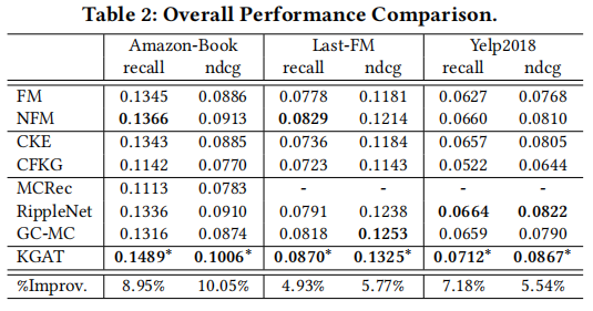
Ϊ��̽���ۺ�����Ӱ��,���߿�����ʹ�ò�ͬ���õ�KGAT-1����,��֮ǰ�ᵽ��GCN��GraphSage��Bi-Interaction,ʵ�������±���ʾ�����Կ���,Bi-Interaction���������:

Reference
[1] �Ƽ�ϵͳǰ����ʵ��. �ʤ��
[2] ��Ȼ���Դ���cs224n-2021�CLecture15: ֪ʶͼ��
[3] ���ϴ�ѧ��֪ʶͼ�ס��о����γ̿μ�
[4] 2022���й�֪ʶͼ����ҵ�о�����
[5] �㽭��ѧĽ��:֪ʶͼ����.�»�����ʦ
[6] https://conceptnet.io/
[7] KG paper:https://github.com/km1994/nlp_paper_study_kg
[8] ����gStore - a graph based RDF triple store
[9] Natural Language Processing Demystified
[10] https://github.com/datawhalechina/team-learning-nlp/tree/master/KnowledgeGraph_Basic
[11] ��һ��֪ʶͼ�ؼ���������. ���ϴ�ѧ ����
[12] cs224w(ͼ����ѧϰ)2021�����γ�ѧϰ�ʼ�12 Knowledge Graph Embeddings
[13] ��ϵ��ȡ���¼���ȡ���밸��:https://github.com/taishan1994/taishan1994 (��������)
[14] ��ĩ����:֪ʶͼ��Ƕ�뷽���о��ܽ�
[15] ��֪ʶͼ��+��ϵ��:֪ʶͼ��+ͼ������
[16] ��֪ʶͼ�ס�˹̹�� CS520������(˫����Ļ)
[17] https://github.com/LIANGKE23/Awesome-Knowledge-Graph-Reasoning
[18] ��̸ͼ�ױ�ʾ:ͼ�����ʾGE��֪ʶͼ�ױ�ʾKGE��ԭ���Ա���ʵ��Ч������
[19] WSDM��23 | ��ҵ�����ƹ�nlp��������
[20] https://github.com/LunaBlack/KGAT-pytorch
[21] �Ƽ�ϵͳ֮����ٻ�ģ������(PART III)
[22] ����ں� | ���Ƽ�ϵͳ����֪ʶͼ��(��)
[23] KGAT_����֪ʶͼ��+ͼע����������Ƽ�ϵͳ(KG+GAT)
[24] KGAT��pytorch��������
[25] ���Ż���֪ʶͼ�ĸ��Ի������Ƽ�ϵͳ